The case-crossover design, introduced by Maclure¹ in 1991, represents an attractive method to investigate the acute effects of an exposure. It has been used, for example, to investigate triggers of myocardial infarction.² In recent years, it has been applied to the analysis of the acute effects of environmental exposures, especially air pollution.^3–6 In the case-crossover approach, a case-control study is conducted whereby each person who had an event is matched with their self on a nearby time period where he or she did not have the event. The subject’s characteristics and exposures at the time of the case event are compared with those of a control period in which the event did not occur. Each risk set consists of one individual as that individual crosses over between different exposure levels in the interval between the two time periods. These matched pairs may be analysed using conditional logistic regression. Multiple control periods may be used.

Applied to the association of air pollution with risk of death, the approach has several advantages. First, it clarifies a key feature of the study of acute response to air pollution. Because in this analysis each subject serves as their own control, the use of a nearby day as the control period means that all covariates that change slowly over time, such as smoking history, age, body mass index, usual diet, diabetes, etc, are controlled for by matching.

The second advantage involves the method of control for seasonal variations in mortality risk. The other possible technique to analyse the association of short term changes in air quality with short term changes in the risk of death or hospital admission has been to collapse the data to daily counts, and use Poisson regression of the daily data.⁷ Because these regressions make comparisons across the full range of data, including multiple years, it is necessary to control for season and long term time trends. While several approaches have been taken to control for the seasonal patterns in the data,^8,9 in 1993 generalised additive models¹⁰ were applied to these analyses,¹¹ and that technique quickly became the standard in subsequent studies.^12,13 These models are attractive because they use smooth curves to control for season (and weather).

Non-parametric smoothing is attractive when one believes a non-linear association exists with a covariate, since it is more flexible than parametric approaches.¹⁰ However, recent studies have reported problems with the algorithms that implement these models.¹⁴ The standard errors of the parametric terms, including the hypothesis variables, are not estimated correctly.¹⁵ Because too small estimates of within location standard errors leads to larger estimates of heterogeneity (the between location variance), recent reanalyses of multi-location studies did not show bias in the estimated standard errors of the combined effect estimates.^16,17

These problems have encouraged reanalysing previous studies to confirm whether the reported associations still hold. Natural splines are a possible alternative, and have been used previously,¹¹ but they have some sensitivity to the locations of the knots for the splines. Details of spline models have been published elsewhere,^10,11 but in essence, they divide a continuous variable into a set of discrete ranges, and fit separate polynomials in each range. The boundary points of the ranges are called knots. Natural splines have recently been applied to a reanalysis of the National Mortality and Morbidity Air Pollution Study (NMMAPS), a large multi-city study of particulate air pollution and daily deaths.¹⁴ There has been a continuing debate over how many degrees of freedom are appropriate to use to control for season, and switching from non-parametric smoothing to natural splines does not resolve this issue. More recently, similar debates have emerged about how many degrees of freedom to use for weather.

The large number of studies of daily changes in air pollution and deaths has been a basis for tighter air pollution standards in both the United States and Europe. The recent questions over the reliability of these estimates have, therefore, considerable public health importance.

The case-crossover design controls for seasonal variation, time trends, and slowly time varying confounders by design because the case and control periods in each risk set are separated by a relatively small interval of time. Bateson and Schwartz^18,19 showed that by choosing control days close to event days, even very strong confounding of exposure by seasonal patterns could be controlled by matching in the case-control approach. Also, because the analysis is of matched strata of days for each individual, it is straightforward to combine events from multiple locations in a single analysis. The difference in seasonal patterns from city to city has prevented this approach in multi-city studies using Poisson regression. This makes the approach an attractive alternative to the Poisson models. While Bateson and Schwartz¹⁹ have shown that the power is lower in the case-crossover approach, this is less of a concern in a large multi-city study. Because the case-crossover approach focuses on individual events, rather than daily counts, it also makes examination of effect modification more straightforward.

While it is straightforward to sample control days in a manner that removes seasonal confounding, there can be a subtle selection bias in these analyses.^19–21 For example, days before the first event serve as control days, but cannot serve as event days, and occasional days with missing data for exposure during the event series can further increase selection bias. Further, Lumley and Levy²⁰ have pointed out that the selection of controls is not independent sampling, since the case day always falls in the middle. This introduces a small selection bias as well. Lumley and Levy²⁰ suggest a time stratified approach, where the control days for a given subject are randomly selected from all days in the same month of the same year. Bateson and Schwartz¹⁹ suggested that maintaining symmetrical control sampling would provide better seasonal control, and demonstrated an adjustment method that gives unbiased estimates. A recent simulation study showed that both approaches give unbiased estimates and unbiased coverage probabilities.²² I have applied both approaches to a multi-city study of particulate air pollution and daily deaths in a study of 14 US cities.

For comparison, I have also analysed those cities using Poisson regression of daily counts, with penalised splines²³ used to control for season and weather. Penalised splines do not suffer the standard error problem of the earlier generalised additive model approaches.

DATA AND METHODS

Most cities in the USA only monitored PM₁₀ once every six days. This can create difficulties in finding control days close to event days. To avoid this, I studied 14 US cities with daily monitoring schedules: Birmingham, AL; Boulder, CO; Canton, OH; Cincinnati, OH; Columbus, OH; Chicago, IL; Colorado Springs, CO; Detroit, MI; Minneapolis/St Paul, MN; New Haven, CT; Pittsburgh, PA; Provo-Orem, UT; Seattle, WA; and Spokane, WA. I chose the metropolitan county containing each city except for Minneapolis and St Paul, where both metropolitan counties were combined and analysed as one city.

Daily mortality

Deaths in the metropolitan county containing each city were extracted from tapes prepared by the National Center for Health Statistics (NCHS) for the calendar years 1986 (when PM₁₀ monitoring began to be phased in by the US EPA) to 1993. Deaths from accidental causes (International Classification of Diseases 9th Revision, ICD9 ⩾800) were excluded, as were all deaths that occurred outside of the city. While deaths were available from 1986, in some cases PM₁₀ monitoring did not begin until later. This results in some variation in the study period by city.

Exposure and weather data

Daily measurements of mean temperature and relative humidity were obtained from the nearest National Weather Service Surface Station for each county (EarthInfo CD NCDC Surface Airways, EarthInfo Inc., Boulder, CO).

Air pollution data for PM₁₀ were obtained from the US Environmental Protection Agency’s Aerometric Retrieval System (AIRS). Many of the cities have more than one monitoring location, requiring a method to average over multiple locations. This study uses an algorithm previously reported.²⁴ To ensure that the exposure measure represented general population exposure and not local conditions affecting only the immediate vicinity of a given monitor, the correlations among all monitors in each county were computed. Monitors within the lowest 10th centile of the correlation across all counties were excluded. While all locations had daily monitoring for PM₁₀ by at least one monitor, some monitors only measure PM₁₀ one day in three or one day in six, and different monitors have different means and standard deviations. I did not want the daily pollution value to change from day to day because of changes in which monitors reported, as opposed to differences in actual ambient levels. In each city the daily mean among monitors for each pollutant was calculated using an algorithm that accounted for differences in the annual mean and the standardised deviations of each monitor as follows. The daily standardised deviations for each monitor on each day were averaged; these were then multiplied by the standard deviation of all of the monitor readings for the entire year, and added back in the annual average of all of the monitors.¹³ I used the air pollution concentration the day before each death as the exposure variable, because the NMMAPS^13,14 study has found that to be the most predictive single day exposure, and presents that exposure metric in most of its publications. The NMMAPS study could not analyse multi-day exposures because most of their cities only measured PM₁₀ one day in six. The use of the same exposure metric facilitates comparisons between the studies.

Analytical strategy

Several analyses were conducted. The basic analysis used conditional logistic regression to analyse the data in each city, in a case-crossover design, using the Bateson and Schwartz method to choose control days.¹⁹ I chose this because our simulations showed it did slightly better in the face of strong seasonal patterns and time trends.

Matched strata were constructed for each subject (that is, death), consisting of the event day (day of death) and 18 matched control days. These days were chosen to be the days 7–15 days before the event day, and the days 7–15 days after the event day. Control days were not chosen closer to the event day to avoid serial correlation in the pollution and mortality data. Control days were chosen symmetrically about the event day because Bateson and Schwartz¹⁸ showed that symmetric control days were needed to control for long term time trends (if present). Navidi²⁵ pointed out that bi-directional sampling is needed to avoid some biases in the case-control study, and does not present any conceptual difficulties as long as the inactivity of the subject after death does not affect the air pollution concentrations. The adjustment method of Bateson and Schwartz¹⁹ was used to address the small selection bias pointed out by Lumley and Levy.²⁰ Briefly, this consists of creating a pseudo-data set with the same exposure variables as in the real data, but with one death on every day. By construction, there can be no association between pollution and the risk of death in this dataset. The estimated coefficient obtained from this pseudo-data set was used as an estimate of the bias, and subtracted from the naïve estimate obtained analysing the real data.

In all analyses, I controlled for day of the week, temperature, and relative humidity. Temperature may be non-linearly related to the risk of death, and so I used regression splines to control for temperature on the day of death and the day before death. These splines used 3 degrees of freedom each. Relative humidity was controlled for in a similar manner.

The first analysis used a two stage approach. A city specific regression was fit using the matched strata from each city. The log odds ratios from those 14 analyses were then combined using the iterative maximum likelihood algorithm of Berkey and coworkers,²⁶ allowing for heterogeneity in effect across city. In this analysis, the splines for temperature could have different coefficients in different studies. The random effects estimate was used in this case, whether or not the random variance component was significant, because the significance test for that component is weak, and I wanted to be sure to incorporate heterogeneity.

Because the control days are chosen close to the event day in the case-crossover analysis, the range of variation of temperature, and the range of its effects, is lower than in other study designs. This suggested that I could aggregate all of the strata together, and analyse the association with air pollution across all 14 cities in a single model. This is an attractive feature of the study design, and constituted the second analysis. It is equivalent to assuming no heterogeneity in response across cities, however.

In the third analysis, I used the time stratified method of Lumley and Levy²⁰ to select control days for each person who died. In addition to matching on season, I also matched on temperature. That is, I chose control days to be days in the same month and year as the death occurred, that also had the same temperature (rounded to degree Celsius). In these analyses, I continued to control for humidity on the same and the previous day, and for temperature on the previous day, using regression splines. Both two stage and single stage analyses were done using the time stratified control selection method as well.

To facilitate comparison with more traditional Poisson regression analysis, I reduced the data to counts of daily deaths, and performed Poisson regressions in each city. These models used penalised splines with 4 degrees of freedom per year for season and 3 degrees of freedom for each weather variable (today’s and yesterday’s temperature and humidity), as well as day of the week dummy variables. The use of a pre-specified fixed number of degrees of freedom in a penalised spline model reduces it to a ridge regression, with well developed methods for estimating standard errors, unlike the problems with generalised additive models.

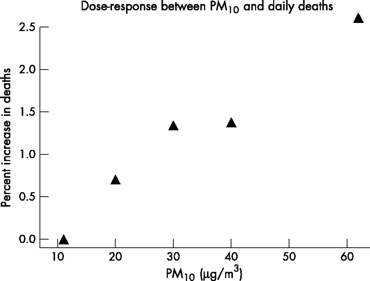
To test the shape of the dose-response relation, I replaced the linear term for PM₁₀ with the indicator variables for days when concentrations were between 15 and 25 μg/m³, between 25 and 34 μg/m³, between 35 and 44 μg/m³, and 45 μg/m³ and above. The days with concentrations below 15 μg/m³ served as the reference level. This model was fit using the single stage method, combining strata across all cities

RESULTS

Table 1 shows the 25th, 50th, and 75th centiles of the distribution of air pollution and weather in each of the 14 locations, as well as the total number of deaths studied in each location. Weather was only modestly correlated with PM₁₀ in these locations, as shown in table 2.

In the two stage analysis, I found a significant association between PM₁₀ and the odds of dying. The magnitude of the association was a 0.36% increase in the risk of death per 10 μg/m³ increment of PM₁₀ (95% CI 0.22% to 0.50%). Combining all the strata and analysing in one stage had little impact on the estimate (0.33% increase, 95% CI 0.19% to 0.46%). Table 3 shows the individual city results. There was no evidence for heterogeneity in the association (χ² = 12.17 on 13 df, p = 0.51), but a random variance component was kept to be conservative.

Table 4 shows the results of further sensitivity analyses. Matching on same day temperature (and continuing to control for humidity and previous day’s temperature) had little impact on the effect estimates, which were in fact slightly larger than those found without matching. Further, the results were not noticeably different from those found using a more traditional Poisson regression analysis.

Figure 1 shows the results of the analysis using categories of PM₁₀ exposure to look at the dose-response curve. There was little evidence of deviation from linearity.

DISCUSSION

Substantively, this analysis confirms that using parametric regression techniques which avoid the software problems in generalised additive model software, one still finds a significant association between daily levels of PM₁₀ and daily deaths. It extends that finding by: (a) doing so using a very different approach, indicating a robustness of the results to type of modelling; and (b) in particular using an approach that avoids having to model seasonal patterns at all, obviating arguments about the complexity of those models.

Methodologically, it shows an approach that has certain advantages over the previous methods applied to multi-city studies. While case-crossover analyses have been reported in single city studies,^3–6,19 this is the first application to multi-city studies in air pollution. The results of the primary analysis are indistinguishable from the results of a Poisson regression applied to the same data. Wherein lie the potential advantages?

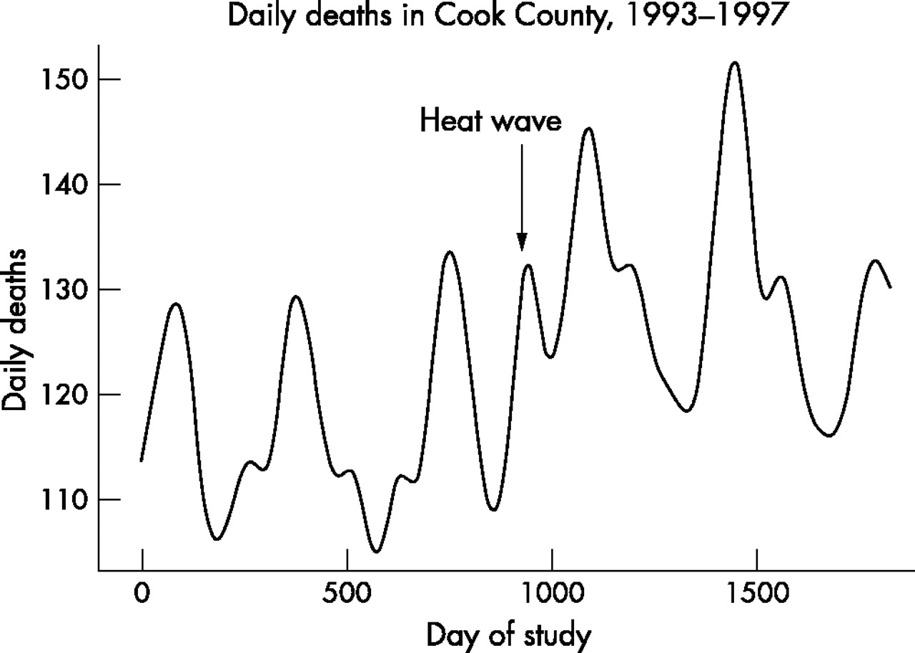
First, case-crossover methods allow the possibility of avoiding arguments about how many degrees of freedom and what functions are necessary to control for season, since seasonal control is done by matching. It also makes the method of seasonal control more accessible to readers less familiar with the literature on splines and smoothing. Matching within two weeks is more intuitive than choosing a number of degrees of freedom per year for seasonal control. Splines and other flexible functions can fit the data in ways not expected. For example, consider a study interested in the immediate effects of ambient temperature on mortality risk. Figure 2 shows the results of fitting a 7 degree of freedom per year spline model to explain seasonality for daily deaths in Chicago during the years 1993–97. In the summer of 1995 there was a serious heat wave in Chicago, which was responsible for an estimated 400 early deaths over a six day period. One can see that the 7 df/year seasonal model is fitting a peak of mortality in the middle of the usual summer trough in 1995. That is, 7 degrees of freedom per year is sufficient to start picking up not merely season, but also the effects of a six day weather episode. This is in contrast to many people’s intuition that it only removes patterns on the order of two months or longer from the data. A standard method of attributing deaths to heat waves is to count the excess over the seasonally expected during the heat wave period. Clearly, this peak in the summer months attributable to “season” will reduce the number of excess deaths that can be attributed to the coincident heat wave by that method. A case-crossover analysis of the effects of temperature that makes sure to choose control days outside of the heat wave period would easily avoid this problem in identifying the temperature effects.

Second, as shown here, for air pollution studies, it is possible to match on temperature as well as season. This offers great advantages. It obviates the arguments about how to control for same day temperature. Also when matching on season and temperature, one implicitly controls for all interactions between those variables.

Temperature is not the only weather variable, and may exert effects with some lags. However, Braga and colleagues²⁷ and Cuireiro and colleagues²⁸ have shown that the largest weather effect is on the same day. Matching can control that portion of the weather’s effects. Further, while there is no explicit matching on lagged temperature, days matched to within two weeks of time and with the same temperature do not differ greatly in temperatures on the previous days. For example, across these 14 cities, the mean standard deviation of the previous day’s temperature within strata (case and control days), after matching by current day’s temperature, was 2.2°C. Hence lagged temperature is indirectly controlled to a substantial extent by matching. The lack of change in the risk estimate for particulate air pollution in these cities comparing matching on temperature with regression modelling to control for temperature indicates that the models adequately controlled for temperature before matching.

An additional advantage of the case-crossover design is the ability to combine information across cities in a single stage model. Because strata of event and control days within subject are matched on season (and weather), it is possible to combine these strata in a single analysis. One example of the possibilities this engenders is the analysis of the shape of the dose-response relation presented in fig 1. While this paper presented a simple approach, more complex analyses, include spline models and smoothing, are available, and in this application need no longer be combined across cities in a two stage model. Multilevel modelling of effect modification by city characteristics is easily incorporated in the single stage model. Effect modification by individual characteristics may also be examined. In the past, this has been done by stratified Poisson regression, such as the identification of diabetes as a potential modifier of the effect of PM₁₀ on hospital admissions for heart disease,²⁹ but identification of characteristics can be more easily incorporated into the case-crossover approach.

Nevertheless, the case-crossover approach does have important limitations. One key limitation is the difficulty in examining associations over longer time periods than a few days. This limits the methods ability to examine either harvesting or associations with longer term exposure. In addition, while Lumley and Levy²⁰ have shown a proper conditional logistic likelihood with time stratified sampling, and Schwartz and coworkers²² have shown both unbiased estimates and unbiased coverage probabilities (and hence confidence intervals), more remains to be learned about the theoretical properties of this approach.

The examination of dose-response in this analysis shows little evidence for a deviation from non-linearity. However, it is important to understand that the range in exposure was not enormous in this study. For example, annual average PM₁₀ concentrations in Athens exceed the highest category in fig 1. Hence non-linearities at higher concentrations cannot be excluded by this analysis. It is also interesting to note the pattern of correlations between PM₁₀ and weather variables in table 2. The Midwestern cities all had moderate, positive correlations between temperature and PM₁₀. This is likely due to the importance of sulphate particles in that region. Sulphate levels, and levels of other long range transported particles, tend to increase on hot days because of increased photochemistry. In contrast, in the northwest part of the country, the correlation was negative, and smaller. This region is less impacted by sulphate. Hence differences in these correlations may reflect different sources and atmospheric processes contributing to exposure.

In conclusion, the reported association between short term variations in air pollution and risk of death has been confirmed in a study of 968 514 deaths using a substantially different methodology than previous studies. This indicates a robustness of the association, and avoids any of the standard error problems of generalised additive models. The case-crossover approach deserves attention in the future for studies of acute health effects of pollution.