Study design

The study involved an initial period of method development and validation. This was followed by two main investigative phases:

• Phase 1: Establishment of the relations between the direct and indirect methods of measuring pollutant exposures. Using a number of volunteer subjects, personal exposure was measured directly through attaching personal samplers to the subjects and estimated indirectly through a combination of microenvironment measurements and activity diaries indicating the periods of time spent by the various subjects in the different microenvironments.

Healthy adult volunteers were recruited for this section of the study. They were requested to go about their everyday life while wearing personal sampling equipment. In addition to this, static equipment was sited in the volunteer's home, in the room most frequently used during waking hours. This was generally a living room, and in the majority of cases was in close proximity to the kitchen.

Eleven volunteers were recruited to undertake this section of the work. They were required to carry out the sampling for 10 day periods and thus incorporated weekend sampling where possible. Sampling was carried out for approximately eight hours per day.

• Phase 2: Investigation of the difference of exposure patterns between susceptible groups of the population and healthy groups. Small panels of susceptible individuals were set up and their exposures estimated through personal sampling of an investigator who shadowed the activity of the susceptible group members. Additionally, microenvironment methods were operated within the homes (and school) of the susceptible groups. The range of exposures within the susceptible groups were compared with those of the healthy volunteers used in phase 1.

Three susceptible subgroups were identified. These were the young, the elderly, and those with existing illness known to increase susceptibility to the adverse effects of air pollutants. People were chosen from within these groups, and their daily lives were shadowed by a researcher wearing the personal sampling equipment as it was not considered appropriate to have them wearing the bulky equipment themselves.

Shadowing was carried out with six children, six elderly people, and six people with existing illness (two with chronic obstructive pulmonary disease (COPD), two with left ventricular (heart) failure (LVF), and two with severe asthma). This was done for six hours a day, for five day periods (Monday to Friday).

The study of the young persons group was carried out in a Year 6 class (approximately 10 years of age) at a primary school in Birmingham. Six children were shadowed during their school day. To do this, slight adjustments to sampling times were made to fit in with the school timetable. Static NO₂ and PM₁₀ measurements were made in the classroom. Static CO measurements were also made, but because of the noise and size of the CO analyser these measurements had to be made in a separate classroom.

Six elderly subjects (aged >65 years) were shadowed during their normal day. In most cases the majority of time was spent in the home, with some time spent at local shops or walking dogs. Static equipment was sited within the home, again in the most frequently used room. Staff at Birmingham Heartlands Hospital recruited the six volunteers with severe disease. Many of these subjects spent much time in their home, although one subject worked full time, and in this case, the shadowing was carried out in the place of work. Static site monitors were placed either in the home or the place of work depending on where the majority of sampling time was spent.

Sampling methodology

Modelling of personal exposure

Carrying out direct personal exposure measurements is costly and time consuming. For this reason, it is important to find other methods of assessing accurately an individual's exposure to pollutants. This can be done in a number of different ways and for the purpose of this study, modelled 5 hour and 24 hour integrated personal exposures were calculated for the susceptible groups (the young, the elderly, and those with existing illness) using the microenvironment measurements and activity patterns collected as a part of this study.

These were calculated from the equation:where C_x = mean concentration in microenvironment x (ppb); and t_x = time spent in microenvironment x (h).

Static monitoring data (phase 1)

In the case of both nitrogen dioxide and carbon monoxide, the mean and range of concentrations were fairly typical of background urban air, representing the ingress of polluted outdoor air into buildings with some additional modification because of indoor sources. In the case of PM₁₀, however, the vast majority of the concentrations greatly exceeded those measured at urban background locations, implying emissions of particulate matter from indoor sources.

Personal monitoring results (phase 1)

For NO₂ and CO, hourly integrated personal exposure data were collected, and from activity diaries filled out during the sampling period it was possible to assign to each data point contributions from the different microenvironments in which the volunteer had spent time. Increases in concentration were observed associated with travel in a car, proximity to roads and, for CO, proximity to a bonfire. The exact contribution from these sources cannot be calculated, as frequently volunteers will not spend the entire one hour sampling period in the same microenvironment. Personal PM₁₀ data were collected over 2–3 day periods, providing an average mass concentration for this period. For this reason it is not possible to identify elevations associated with individual sources or activities.

Table 2⇓ shows a summary of all the personal data collected as part of the exposure study. Average concentrations shown for NO₂ and CO were calculated from one hour samples over the entire sampling period, while the PM₁₀ data were from 2–3 day exposures.

Comparison between personal and static concentrations (phase 1)

Because of the nature of this phase of the work, it was not always possible to obtain directly comparable data as the healthy volunteers used in this phase of the study often spent much of their time away from home, while static data were collected only in the home. This, coupled with problems encountered with the Scintrex analyser, means there are no directly comparable data available from this section of the work for NO₂.

Figure 1⇓ shows all the directly comparable data for CO. It can be seen that most of the data lies close to a trend line with a few outliers. When volunteer information is studied, these outliers can be clearly associated with environmental tobacco smoke (ETS). For non-smokers, a gradient approaching 1 is observed with a near zero intercept.

• Download figure
• Open in new tab
• Download powerpoint

Figure 1

Plot of directly comparable personal and static carbon monoxide concentrations from the phase 1 exposure study.

Table 2⇑ shows averaged phase 1 PM₁₀ data for each volunteer. Comparable sets of personal and static PM₁₀ data, specifically those from sampling periods when the volunteer has spent the majority of time in the home and hence in the same microenvironment as the static sampler, were analysed, excluding data for smokers (for whom a great increase in particle concentration about the person might reasonably be expected). A good relation was observed (R² = 0.90), with a gradient of 1.28 and an intercept of personal exposure of 33 μg/m³ (n = 9).

Personal sampling data (phase 2)

Table 3⇓ gives a summary of the personal data acquired from the different microenvironments. Average concentrations shown for NO₂ and CO were calculated from one hour samples over the entire sampling period. Average concentrations shown for PM₁₀ were measured gravimetrically from one sample collected over the sampling period. Linear regression relations were calculated between static concentration and personal exposures for each of the different microenvironments.

Results from shadowing of susceptible groups

Table 4⇓ presents the results of regression analyses between personal exposure (y) and static concentration (x) measurements. Because of problems with the Scintrex analyser, static NO₂ data were collected for only three of the periods of shadowing.

Table 5⇓ presents results from the shadowing of elderly subjects. Static data for nitrogen dioxide were collected both with the Scintrex continuous instrument and with static Sep-Pak cartridges. The latter are directly comparable with the method used for personal nitrogen dioxide monitoring and do not require the lengthy stabilisation periods which the Scintrex needed. The regression relations obtained solely using the Sep-Pak cartridges are therefore more credible.

Table 6⇓ presents data for subjects with pre-existing illness. Regression relations for nitrogen dioxide were also omitted as these most probably reflect of inadequate instrument stabilisation rather than the true relation between static and personal sampling results. Data collection for carbon monoxide was only possible for two of the subjects. In both cases strong relations between static concentrations and personal exposure were found. For PM₁₀, in all but one case, the personal exposure considerably exceeded the static measurement, typically by a factor of around 3.

Modelling of personal exposure

Because of initial difficulties with the Scintrex instrument, data for nitrogen dioxide were not considered sufficiently reliable for this exercise. In the case of both CO and PM₁₀, one concentration, based on the mean of measurements, was adopted for each microenvironment. The relation between personal (y) and static (x) PM₁₀ of y = 1.17x + 17 was used to correct the average static concentrations in each microenvironment to an equivalent personal concentration. Five hour integrated personal exposures to CO and PM₁₀ were calculated for the young, the elderly, those with severe asthma, COPD, and LVF, and the “healthy” group from phase 1 based on activity diaries kept by the subjects. Actual measurements of personal exposure for the different groups were then converted into concentration.hour units (see table 7⇓).

Twenty four hour integrated personal exposures to CO and PM₁₀ were calculated for the young, the elderly, and those with severe disease (as a group) based on activity diaries filled out by 10 volunteers from each of these groups. For the young, a whole class (30 pupils) filled in the diaries as it was thought that this was more representative than selecting individuals; from these diaries, 10 were selected from those that were filled out correctly. In addition, two of the pupils suffered from asthma and their diaries were analysed separately. Tables 8 and 9⇓⇓ give the results of this analysis.

Shadowing

NO₂ data for shadowed children showed variable but generally statistically significant relations between personal and static concentrations, although it was only in later measurements that the same method was used for both static and personal concentrations so that wholly reliable relations were derived. These data should therefore be looked on with some caution. The data for carbon monoxide should, however, be reliable, and it is encouraging that three of the four regressions indicate slopes quite close to 1, and intercepts that are generally quite small in relation to the concentrations. This is strongly suggestive of carbon monoxide personal exposures closely parallelling static concentrations within the school. Turning to PM₁₀, the comparison of personal and static results (table 4⇑) shows that during two of the three periods for which data are available, the static concentration exceeded the personal concentration, which is unusual for comparisons of this type.

For the pensioners there were also mixed results. For two (OAP 5 and OAP 6), NO₂ showed a high correlation coefficient and a slope close to 1. The regressions for carbon monoxide on these two subjects were not good, while those for subjects OAP 2 and OAP 3 showed both a high correlation coefficient and slopes reasonably close to 1. The divergence in the apparent behaviour of these pollutants is unexpected, but probably explained by a greater range of concentrations for NO₂ than for CO, allowing more effective regression. The results for PM₁₀ show appreciably higher personal concentrations than static (table 5⇑). The difference is most notable for subjects OAP 1, 3, and 4, who were either smokers or living with smokers. The presence of smokers caused a large increment in the personal exposure concentration (see table 5⇑), but not the static concentration. It is possible that the siting of the static monitor within the home was not such as to reflect fully the influence of ETS, which was relatively localised. Because of the rather anomalous nature of the data for the ETS exposed subjects 1, 3, and 4, these data points have been omitted from subsequent pooled data analyses.

Comparison between all personal and static measurements

For the statistical analyses on single sets of data shown above, the data are frequently clustered within a narrow range of values, or of a limited sample size, providing unsatisfactory regression and R² values. This section discusses comparisons between all comparable personal and static measurements made as part of this project. The increased sample number and range should improve the power of the regression analysis to identify relations.

Carbon monoxide

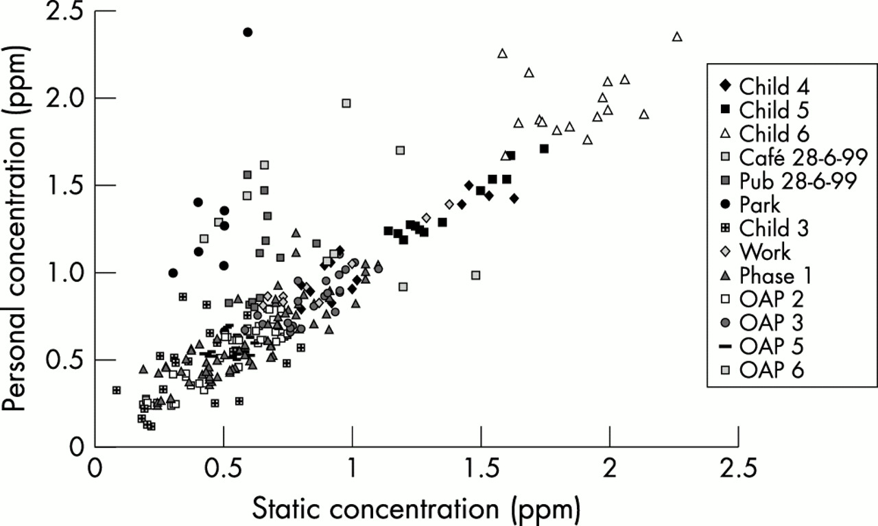
When all the carbon monoxide data were pooled, a clear trend appeared in the data, with a near one-to-one relation between static and personal concentration data. There were, however, some points lying well off this line. To determine whether these outliers belonged to specific subsets of data, the pooled data were replotted with individual subsets identified (fig 2⇓); ETS affected samples were omitted as atypical of normal ambient exposures. The anomalous data fell into three distinct classes: those collected at the park, café, and bar. In the case of the park, the static data were taken from a Birmingham City Council mobile unit sited close to the park, but across a road. A possible explanation is that the park was downwind of the road and experiencing higher concentrations, which were reflected in increased personal exposure values relative to measured static concentrations. The café and bar data may well be indicative of static measurements being made in little occupied areas of the café and bar influenced by extraction systems, whereas the personal data were collected in the more heavily occupied areas and were more subject to smokers, etc. If the data from these three sources are removed from the comparison, the plot shown in fig 3⇓ results. This shows an excellent relation between personal and static carbon monoxide relations with a very high regression coefficient, a slope of 0.97, and a near zero intercept. Clearly, in the case of carbon monoxide, personal exposures reflect microenvironment concentrations extremely well in many situations, the exceptions being identifiable circumstances that can result in high spatial variability within a microenvironment. Such circumstances include proximity of strong sources (notably ETS) and localised ventilation effects.

• Download figure
• Open in new tab
• Download powerpoint

Figure 2

Plot of personal versus static carbon monoxide concentrations in terms of sampling location.

• Download figure
• Open in new tab
• Download powerpoint

Figure 3

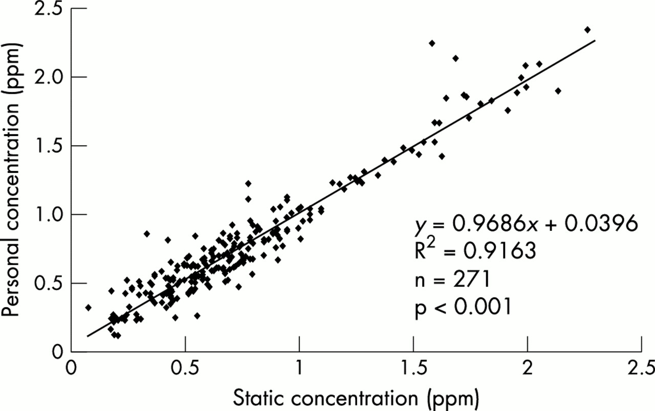
Plot of personal versus static carbon monoxide concentrations for phases 1 and 2, excluding data from the park, café, and bar, and samples affected by passive smoking.

Carbon monoxide is perhaps the ideal analyte for this kind of study. It is chemically rather unreactive, and while spatial inhomogeneities arise as a result of local source emissions, concentrations within buildings are likely to be fairly uniform as a result of the absence of strong indoor sources and sinks, other than in the presence of smokers, gas fuelled domestic appliances, or localised ventilation. It is therefore unsurprising that after the removal of a small number of explainable outliers, the relation between measured personal exposure to carbon monoxide and the associated microenvironment concentration is excellent. This gives confidence that for carbon monoxide, measurement of microenvironment concentrations is generally an excellent predictor of personal exposure.

Nitrogen dioxide

Many of the early microenvironment concentration data in this study were invalid because of problems with the measurement instrument, which was very poorly suited to the rigours of frequent movement and switching on and off. However, the personal exposure measurement technique for nitrogen dioxide developed in the course of this study proved to be highly robust and gave excellent results. Data from samples collected using statically sited Sep-Pak cartridges were compared with personal measurements, as shown in fig 4⇓. A strong relation was observed, with a gradient of 1.0 and a small intercept. The intercept (2 ppb) could possibly be related to exhalation of nitric oxide, which in some circumstances could be oxidised to nitrogen dioxide by ozone. This dataset, then, although smaller than that for carbon monoxide, confirmed a very close relation between personal exposure and the associated microenvironment concentration for nitrogen dioxide. Again, this gives confidence that measurements of microenvironment concentration are an excellent surrogate for personal exposure estimation in that microenvironment.

• Download figure
• Open in new tab
• Download powerpoint

Figure 4

Plot of personal versus static concentrations of nitrogen dioxide measured by the Sep-Pak cartridge technique.

PM₁₀

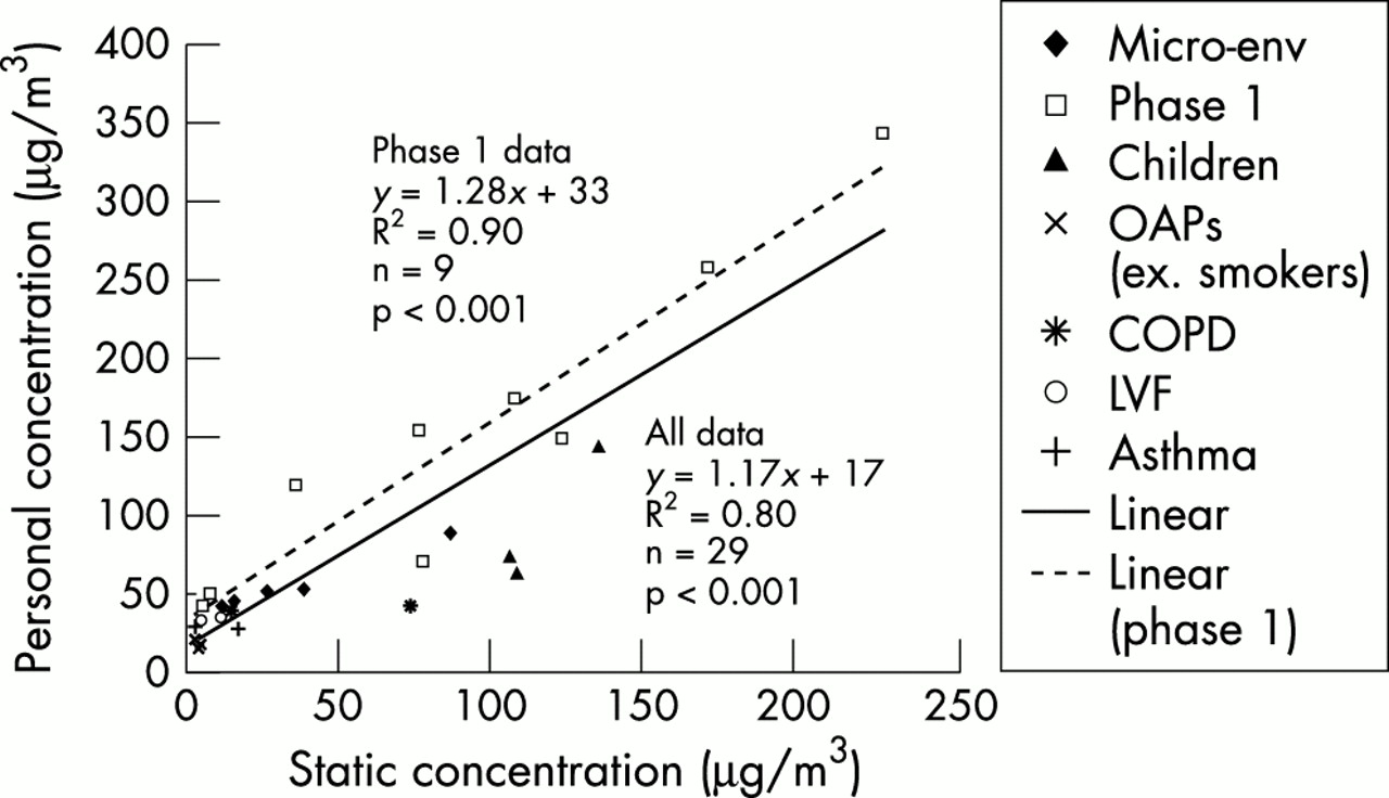
When collecting personal samples of PM₁₀ gravimetrically, it is difficult to build up a large comparable data set because of the long sampling periods associated with the personal method. A data set sufficient for statistically meaningful analysis was acquired, however, and this is plotted in fig 5⇓. For all pooled data a gradient of 1.17 was observed, with an intercept (± 1 SD) of 17 (10) μg/m³. This intercept is lower than has been observed in a previous project involving healthy adults¹⁴ where an intercept of approximately 30 μg/m³ was found, and considerably smaller than that determined in the American PTEAM and THEES studies for PM₁₀.^18,19 However, when the data from the healthy adult volunteers in phase 1 are analysed alone, a line of intercept 33 μg/m³ and slope 1.28 is obtained, comparable to the value from the previous study, and suggesting that the personal cloud associated with the susceptible groups in this study is typically lower than that of healthy adults.

• Download figure
• Open in new tab
• Download powerpoint

Figure 5

Plot of personal versus static concentrations for PM₁₀.

In a study conducted in the Netherlands, the median intercept in the relation between personal PM₁₀ and indoor PM₁₀ measurements was 13.1 μg/m³ with a median slope of 1.00 in measurements on 50–70 year old adults after excluding days with exposure to ETS.²⁰ Here, too, the presence of less active elderly individuals may account for the reduced personal cloud. Most other studies of personal exposure to particles (for example, Lachenmyer and Hidy²¹ and Williams and colleagues²²) have used particle size fractions smaller than PM₁₀ and are therefore not directly comparable with this study. It can be seen from fig 5⇑ that the personal exposures to PM₁₀ of susceptible groups tend to fall in the lower part of the range of exposures found for all volunteers. These two observations suggest that PM₁₀ exposures of the susceptible groups may be lower than those of the population as a whole. When the data were analysed according to their group, it appeared that shadowing very active groups, such as the children, may underestimate their personal exposure, as although the “shadower” is in the vicinity of the child, they may not be as active.

For the pooled data, then, PM₁₀ personal exposures correlate well with microenvironment concentration, and can be modelled once a value for personal cloud contribution is included. As the personal cloud effect is by no means yet fully understood, it is not possible to comment on the significance of this difference. Furthermore, while the immediate source of the personal cloud is reasonably comprehensible, the original source apportionment of the particles contributing to the personal level is not known. It is likely to vary considerably, both between individuals and within individuals over time, but the complexity is such that exploring this route further will prove challenging.

Modelling

For both CO and PM₁₀ the modelled concentrations are of an appropriate magnitude, but measured exposures show a far greater range than modelled exposures. This result is most probably a reflection of variability in actual microenvironment concentrations, which the modelling study did not account for as it adopted a single value of concentration for each microenvironment type. Calculated exposures for each group were similar, with very little difference between weekday and weekend exposures, except for the young (schoolchildren) for PM₁₀. This is a result of the fact that time spent in the home clearly dominates the activities of the susceptible groups. The influence of smoking in the home is grossly underestimated for PM₁₀.

While this modelling method is able to simulate the general magnitude of a personal exposure measurement, the modelled and measured personal exposure are not well correlated, generally because the modelled personal exposure is unable to reflect the variability of measured personal exposures occasioned by the spread of concentrations within given microenvironments. Thus, the modelled values show a much smaller range than those measured. However, in terms of representing mean exposures, the modelling approach appears valid.

Clearly for carbon monoxide and nitrogen dioxide, if microenvironment data were available from the homes and other environments occupied by susceptible subjects, it would be possible to model their personal exposures reliably. However, the use of generic microenvironment data derived from the pooling of a number of groups leads to a blurring of the genuine differences in personal exposures. Thus, modelled exposures to nitrogen dioxide and carbon monoxide vary little between individuals, while measured five hour personal exposures vary quite substantially. It is clear that for these pollutants modelling can be very representative of true exposures if appropriate microenvironment data are available, but in the absence of such data, the uncertainty of estimates is increased in a manner related to the variability in concentrations within ostensibly similar microenvironments. This conclusion is true also for particles, although the situation is complicated somewhat by the personal cloud effect and the heavy influence of passive smoking on personal exposures, which was not well reflected in our data on static microenvironment concentrations.

When comparing our susceptible groups with healthy subjects, it is clear that for the measured personal exposures, the less active susceptible group individuals, most notably the retired subjects from non-smoking homes, received lower personal exposure doses, especially to particulate matter, than were typical for the healthy adult group. For the schoolchildren, however, their level of activity is extremely high and their school is in a relatively polluted location, and therefore their personal exposures were comparable with, or higher than those of our healthy subjects. The value of the microenvironment modelling approach over estimates of exposure based solely on outdoor monitoring station data is illustrated by the findings of Linaker and colleagues.²³ In a study of British schoolchildren they found no significant correlation between weekly mean personal exposures to nitrogen dioxide and mean concentrations, measured outdoors only, for the corresponding periods. Dimitroulopoulou and colleagues,²⁴ in modelling exposures to nitrogen dioxide, have highlighted the importance of gas cooking as a source of exposure and estimated that the contribution of outdoor exposure to annual mean NO₂ exposure is not dominant, varying from 5% to 24%.

Overall, it is clear that personal activity patterns can strongly influence pollutant personal exposure, and that relatively inactive subjects may well receive lower personal exposures to the air pollutants considered in this study if they spend much of their time inactive within the home.