A growing body of epidemiological research indicates adverse effects of outdoor air pollution on birth outcomes,1 2 such as low birth weight, preterm birth and intrauterine growth retardation. Studies of birth outcomes have used different methods to estimate exposure, including nearest monitor,3 interpolation4 and traffic-based metrics,5 or, for small study populations, short-term personal sampling.6 7 Various studies have reported associations between modelled estimates of traffic-related air pollution and adverse birth outcomes,5 8 but these models have not yet been evaluated.

Spatial variability in air pollutant concentrations between cities,9 10 between urban and rural areas,11 and within cities12 has been demonstrated. Recent epidemiological studies have identified the importance of capturing within-city spatial variability in air pollution exposure.13 14 Specifically, studies of traffic-related air pollution have used proximity (ie, living near a busy road),15 traffic volume or density measures5 16 or land-use regression (LUR)17 models as exposure indicators. LUR models use a combination of outdoor measurements and geographical variables to estimate within-city variations in traffic-related air pollution.18 19 Generally, traffic-related air pollution exposure indicators incorporate little or no temporal variability and are used to assess impacts of chronic exposures. A few evaluations of “living near a busy road”20 or traffic density and urbanisation measures,21 as indicators of personal exposure in children, demonstrated contrasts in personal exposure using these metrics. No published studies have evaluated LUR estimates of exposure against personal measurements. A recent evaluation of the use of a small number of ambient monitors to predict population exposure to air pollution in France showed little association between ambient monitors and personal measurements.22^–24 These authors called for caution in using monitor-based approaches in epidemiological studies of long-term exposure (those exploiting spatial contrasts).22^–24

In evaluating air pollution exposure assessment methods for epidemiological studies we suggest some key questions: First, how well do exposure models estimate personal exposure? Secondly, can the ability of models to account for spatial effects be improved by including personal mobility data if available? For example, although people spend 60–80% of their time at and/or near home,25 including subject-level mobility, such as time spent at work or in transit, could improve exposure assessments.26 27 Thirdly, how well do models account for temporal variability (ie, changes in ambient concentrations over time)? Depending on the health effect being studied, either spatial or temporal precision may be particularly important for detecting associations. Air pollution exposure assessment methods commonly used in large epidemiological cohort studies have rarely been evaluated against personal sampling. Accordingly, we collected short-term personal air pollutant measurements and mobility data for a sample of pregnant women and compared these to their modelled concentrations using interpolated ambient monitoring data and LUR models. Using repeated samples per subject, we examined two intermediate term (monthly) exposure models’ ability to predict measured short-term exposures. We attempted to compare the models’ abilities to predict the spatial and temporal components affecting measured personal exposures.

METHODS

Study subjects

We studied a sample of 62 pregnant women living in the central Vancouver metropolitan area in 2005–2006 (population of 1.3 million over 1500 km²). Vancouver benefits from a temperate climate year round, has a relatively healthy and active population, low smoking rates (15% across the province of British Colombia) and high incomes (2003 average income per tax-filer was C$47 000 per year). The inclusion criteria were women who self-reported as healthy and experiencing low-risk pregnancies and non-smokers living with non-smokers. We recruited through prenatal classes, word-of-mouth and posters. The study protocol and material were approved by the University of British Columbia Behavioural Research Ethics Board (#B05-0441).

Exposure measurement and estimation

For each study subject, we generated estimates of exposure to ambient nitric oxide (NO), nitrogen dioxide (NO₂), fine particulate (PM_2.5) mass and filter absorbance, using three approaches: (1) personal sampling, (2) interpolated ambient monitoring measurements and (3) previously developed LUR models.28

Personal exposure measurements and activity recording

Each woman carried personal air monitoring equipment and a global positioning system (GPS) datalogger in a small backpack or shoulder bag (with the air monitors attached to the shoulder strap in the breathing zone), and completed a self-administered time-activity diary during each 48 h sampling session. Subjects completed one to three sampling sessions each (one per trimester); most were in their second trimester when recruited, and thus completed only two sampling sessions. In total, there were 127 sampling days with one to four subjects monitored per day; sampling was conducted from September 2005 to August 2006.

We measured personal fine particles with personal environment monitors (PEM) (MSP, Shoreview, MN, USA). The PEM was loaded with a pre-weighed 37 mm Teflon filter (Pall, East Hills, NY) connected to a battery-powered sampling pump (Leland Legacy, SKC, Eighty Four, PA) set to 5 l/min flow rate. This flow rate, resulting in a 50% cut point of 2.2 μm, was used to collect a sample more representative of traffic-combustion generated fine particles. Triplicate mass measurements were made in a temperature (23°C (SD 0.77°C)) and humidity-controlled (34% (SD 3%)) weighing room as described previously.29 The limit of detection, calculated as three times the standard deviation of the laboratory blanks, was 1 μg/m³ based on a 48 h sample.

After weighing, we measured the reflectance of each filter (Smoke Stain Reflectometer, Diffusion Systems, London, UK) and calculated the absorbance (SOP ULTRA/KTL-L-1.0).30 NO and NO₂ were sampled with Ogawa passive samplers (Ogawa, Pompano Beach, FL) and analysed by ion chromatography. Duplicate sampling indicated a precision of 5% for NO and NO₂ measurements by the Ogawa badges. Limits of detection were 0.1×10⁻⁵ m⁻¹ for absorbance, 8.8 ppb for NO and 4.5 ppb for NO₂.

GPS dataloggers (BlueLogger, DeLorme, Yarmouth, ME) fitted with a long-life battery pack (Alti-tech, Vancouver, Canada) recorded latitude, longitude, time and speed every 5 s while a GPS signal was detected (manufacturers’ reported accuracy ±20 m with full signal). We verified the GPS signal at the start of each session but did not ask subjects to check the signal during the session to avoid overburdening them and to reduce potential bias. We also wanted to evaluate the technology’s application in exposure studies when participants were specifically instructed to ignore the equipment.

In the activity diary, subjects recorded their locations (indoors at home/work/other, outdoors, or in transit) at 0.5 h intervals and we calculated the percentage of time each subject spent in each microenvironment. For GPS route data, points within 350 m of home and 400 m of work were identified, and we calculated percentages of time spent at home and at work from these data.

Geocoding addresses and postal codes

Generally, only postal codes are available in population-based epidemiology studies due to privacy concerns. Therefore, for each subject, we geocoded the home and work address, as well as the postal code centroid, using ArcGIS/ArcMap v 9.1 (ESRI, Redlands, CA, USA), the CanMap Streetfiles, 2001 (DMTI Spatial, Markham, Canada) road network and CanMap Multiple Enhanced Postals (DMTI Spatial). In Canadian urban areas, postal codes can represent an area as small as an apartment building or a block face. Since geocoding may mis-locate addresses for large building footprints, we obtained land parcel data (lot boundaries and addresses) from the municipalities (2004–2005) in the study area and combined these with attribute data from BC Property Assessment.31 All address points were adjusted to the centre of the street-facing portion of their respective land parcels.

Exposure estimates using ambient monitoring data

We extracted hourly PM_2.5, NO and NO₂ measurements from all ambient monitoring stations within 50 km of the subjects’ homes (11 stations for NO/NO₂, six stations for PM_2.5). All stations used consistent methods: chemiluminescence for NO/NO₂ and TEOMs for PM_2.5.32 We assigned ambient monitor data to subjects’ home postal codes using: (1) values from the nearest station and (2) an inverse distance weighted (IDW) interpolation (1/distance²) of the nearest three stations. Measurements were averaged for the 14 days before and after the personal sampling to generate a “monthly” estimate (table 1). Spatio-temporal comparisons and visual representations of LUR and ambient monitor methods for this study area are reported elsewhere.33

Exposure estimates using LUR models

The LUR models28 generate raster (continuous) surfaces (10×10 m resolution) covering the whole of the Greater Vancouver Regional District. Briefly, the models were based on a saturation sampling campaign (112 locations for NO, NO₂; 25 locations for PM_2.5 mass and absorbance). Geographical predictors representing road density, land use, population, elevation and traffic density were used in regression models to predict measured concentrations and generate surfaces from which estimates of concentration at any location in the study area could be obtained. The models used in this study were based on measures of road length and population density. R² values for the models (using geographical predictors) were 0.62 (NO), 0.56 (NO₂), 0.52 (PM_2.5) and 0.39 (absorbance) and validation R² values (comparisons to independent monitors at 16 sites for NO/NO₂ and eight sites PM_2.5) were 0.49 (NO), 0.69 (NO₂) AND 0.09 (PM_2.5). The surfaces were smoothed to decrease the resolution to 30×30 m to avoid small errors in geocoding resulting in large numerical changes in exposure estimates.

A unique feature of these models was the addition of ambient monitoring network data from 1998–2004 to generate adjustment factors for monthly temporal variation. These adjustment factors assume that the spatial pollution patterns remained the same, and raised or lowered the entire model surface relative to an annual average. These monthly adjustment factors were applied to the model surfaces, therefore generating LUR exposure estimates for this study that corresponded to the same month as the personal samples, for each subject-sampling session combination. Both annual and monthly-adjusted surfaces were used for all pollutants except “absorbance” (no monthly trend was applied, by design, because ambient absorbance did not vary consistently by season) (table 1).

We also incorporated “mobility” indicators into the LUR model estimates in this study, using the time-activity and GPS route data. Thus, we generated LUR exposure estimates based on home location only (ie, assuming the subject spent 100% of time at home), home+work locations (weighted by the percentage of time spent at home and work from the participants’ time-activity diary, assuming that the home and work time summed to 100%), and estimates based on the detailed GPS route data (taking into account the full range of locations for each participant during a sampling session). This last was done by extracting the LUR model values for every GPS route point and then averaging the time-weighted estimates for every GPS point in a route. This approach reflects all of the subjects’ mobility during their sampling session and was used only for sampling sessions with “complete” GPS route data (n = 35). To determine “complete routes”, we calculated time gaps between each GPS point (average signal precision was ±30 m when signal was established). Routes were excluded if there were large time gaps (>16 h) or a combination of space and time gaps between points.

Two sets of home and home+work estimates were generated: one based on address location and the other based on postal codes.

Statistical analysis

Data were analysed using SAS-PC v 9.1 (SAS Institute, Cary, NC). All personal measurements were compared against modelled estimates using Pearson’s r correlations. We also created linear regression models for each pollutant with personal exposure (log-transformed) as the dependent variable, using mixed effects models, to examine the ability of exposure estimates to explain different components of the variability (between- and within-subject) in personal measurements, while controlling for repeated measures among subjects.

RESULTS

Of the 62 women in the study, 55 completed two samples and, of those, 10 completed three samples. Subjects with only one sample (n = 7; due to miscarriage, early delivery, moving out of the study area or withdrawal from study) were still included in the analysis. Subjects were primarily white (82%), with a mean age of 32 years, highly educated (90% university educated) and with a median family income of C$60 000–80 000 per year. A total of 127 samples were collected between October 2005 and August 2006 (31% in winter, 39% in spring, 17% in summer and 13% in fall). The mean distance from participants’ home to work was 6.3 km (range 0.7–21 km). There were 13 women who worked from home or did not work.

Since LUR exposure estimates based upon addresses were very highly correlated with those based upon postal code estimates for all pollutants (home: Pearson’s r = 0.90–0.96; work: Pearson’s r = 0.87–0.97), only postal code results are presented. Postal code information is more commonly available for population-based cohorts. Not surprisingly, given monitor density and 1/distance² weighting, estimates based on the nearest ambient monitor were very similar to those based on inverse distance weighting (IDW); therefore results are reported for IDW only.

Personal exposure measurements were higher and more variable (table 2) than LUR or ambient monitor (IDW) exposure estimates. LUR estimates had greater variability and covered a wider range compared to the monitor-based estimates. This is expected for several reasons: LUR incorporates higher spatial resolution, monitor-based estimates are constrained by the range of the (relatively few) monitoring sites, and the monitor-based sites are primarily urban background sites which will suppress some variability.

For the 35 samples with complete GPS route data, the percentage of time calculated to have been spent at home and work was highly correlated with percentage estimates based on activity logs (home: r = 0.96; work: r = 0.88). Six participants worked at home but coded their activities as “work”, which may account for the observed lower correlation for work activities. Similarly, for this same subset, mobility-adjusted LUR exposure estimates (using full GPS route data) were highly correlated with home-only estimates (r = 0.83–0.92) and very highly correlated with the home+work estimates (r = 0.94–0.98) for all pollutants.

Figure 1 shows scatter plots and simple correlations between personal monitoring results and each of the following exposure estimates: estimates based on ambient monitors (monthly, with inverse distance weighting) and LUR (home-based estimates). Only NO demonstrated moderate correlations using all approaches to exposure estimation.

• Download figure
• Open in new tab
• Download powerpoint

Figure 1 Scatter plots and Pearson’s r correlations (and p values) for comparisons between personal measurements (n = 127) and exposure estimates using land-use regression (LUR) and ambient monitoring stations inverse distance weighted.

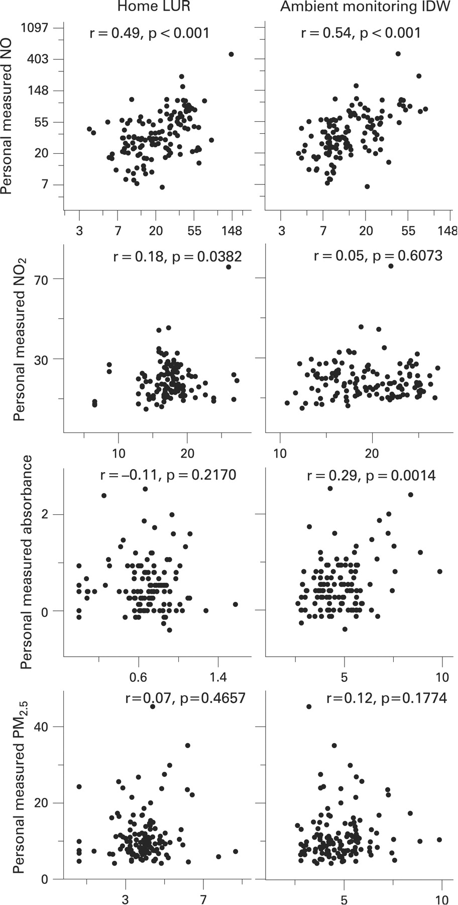
Mobility effects

LUR exposure estimates using home and work locations (table 3) were slightly more highly correlated with personal measurements for NO (r = 0.55) and NO₂ (r = 0.28) than using only home location. For the subset of data with full GPS routes (table 3), using route-based (GPS) LUR estimates showed only slight improvement over the home+work estimates when compared to personal measurements (NO: home+work r = 0.77, GPS r = 0.78; NO₂: home+work r = 0.57, GPS r = 0.66; absorbance: not significant; PM_2.5: home+work r = 0.45; GPS r = 0.47). The correlations were stronger for all pollutants when analysing only the subjects with complete GPS data. However, we noted that on sampling sessions with complete GPS route data, subjects spent significantly more time at home than on the sessions with incomplete GPS route data. When stratifying to subjects who spent more time at home (>65%), the LUR and monitor-based estimates were more strongly correlated with the personal measurements than when using all samples (eg, for NO home LUR: r = 0.72, NO monitors: r = 0.59). The normalised root mean squared errors (NRMSE) show similar trends across the pollutants, the lowest error (7–10%) for NO indicating the trends are strongest for this pollutant. Higher NRMSEs when stratified by mobility are likely due to smaller sample sizes. As the data were log-transformed for analysis, we converted the residuals to the untransformed domain before calculating the RMSEs and normalised the results using the true measurement range thus giving the NRMSE (a percentage) for ease of interpretation.

The mixed-effects regression results (table 4) show the proportion of variability in personal measurements explained by the various exposure estimate “predictors”. If an exposure estimate explains some of the variability in the personal measurements, a reduction in the variance component is expected, compared to a model with no exposure predictors (baseline model). The within-subject variance reflects differences in exposures measured on the subject’s repeated samples, differences expected to be dominated by temporal changes in ambient pollution but also affected by variations in subjects’ mobility or the impact of indoor sources between sampling days. The between-subject variance we expect to be dominated by spatial differences in pollution. In table 4, the within-subject variance component for NO showed little change with different exposure estimates. Since both estimates include the same temporal trends but different spatial characteristics, we conclude that this within-subject variance is dominated by temporal changes in ambient concentrations. For between-subject variance, more variance is explained for NO when work location is incorporated (from 4% to 20%), which supports the hypothesis that this variance is dominated by spatial effects.

Overall, the variance components show similar patterns to the correlations but inform us about how the exposure estimate contributes to predicting the variability in personal data. An increase in within-subject variance suggests that temporal effects are important, whereas an increase in between-subject effects suggests importance of spatial components. The LUR approaches are intended to detect intra-urban spatial differences in exposure, so improving our estimates spatially (ie, by including work location) should increase the ability of the LUR model to predict between-subject differences. In the case of NO and (weakly) NO₂, we observed an increase in variance explained by the LUR model with a more spatially refined estimate. The results for absorbance and PM_2.5 show that the weak correlation (fig 1) of the personal measurements with ambient monitoring data was dominated by within-subject effects likely caused by temporal shifts in ambient pollution. In addition, for these pollutants the between-subject variance was small overall, likely from the low intra-urban spatial variability in concentrations.

The fixed-effect (slope) values from the regression models in table 4 describe a predicted change in the personal sample (dependent) for a change in the exposure estimate (independent) adjusted to the interquartile range (IQR) of that independent variable. These values (table 5 in the online appendix, see supplementary data) are reported as a percentage increase (due to the log-transformation of the dependent variable): for NO, 61% increase with an IQR increase in LUR and 41% increase with an IQR increase in monitor-based estimates (IDW). There was a marginal increase in slope using NO LUR home+work compared to home alone, suggesting that controlling for mobility increased our ability to predict personal exposure using outdoor LUR modelled NO.

Comparing pollutants

Overall, NO models performed best at explaining the spatial (between-subject) variability in personal exposure in this population. For NO₂, annual LUR estimates explained a modest amount of the spatial variability only. In comparing the ability of ambient monitors to predict personal measurements for different pollutants, NO explained more of the between-subject variance than PM_2.5 (table 3) or absorbance; NO₂ was not at all associated.

DISCUSSION

This study is the first to evaluate LUR models as predictors of personal exposure in any study population. The unique focus on personal exposures of pregnant women has also increased exposure data for this potentially vulnerable population. We found that LUR models showed the strongest ability to predict personal measures for some pollutants (NO and NO₂), while ambient monitor estimates were also predictive in some cases (NO, absorbance, PM_2.5). Including mobility, based on work location, improved exposure models.

Evaluation of LUR estimates

Focusing on LUR, we saw moderate correlations and an increasing slope based on the fixed effect estimates from regression models where we controlled for repeated measures among subjects. For NO₂, only annual average LUR values were modestly associated with personal results. While both the NO and NO₂ models were developed using the same number of samples and have similar R² values, only NO showed a strong relationship with personal measurements in this study. Considering only the annual LUR values, NO had much greater spatial variability (higher SD) than NO₂. The surfaces also show less distinct spatial variation for NO₂ than NO (less transitions in colour/shading).28 33 This result was expected, given that NO₂ requires atmospheric transformation, whereas NO is a primary emission. We suspect that the NO₂ signal from traffic is obscured by the effects of indoor sources and its lower spatial variability relative to NO.

We saw little relationship between personal measurements and LUR estimates for particulate pollutants (absorbance, PM_2.5), likely because of the low spatial variability of these pollutants in our area,29 the fewer sites (compared to NO/NO₂) sampled when developing LUR models, and the resulting lower LUR model and validation R² values.28

Evaluation of spatial proximity to roads

Several studies have also demonstrated that differences in traffic intensity and/or living near a busy road can be correlated with personal measurements (NO, NO₂ and/or absorbance). Van Roosbroeck et al20 found an increase of 77% (unadjusted for indoor sources) in home outdoor NO (but no significant increase for NO₂) and 38% in personal absorbance for children living near a busy road (within 75 m of road with 10 000 cars/day) in a study of 40 children in the Netherlands compared to children living at urban background locations. In our study, we found small and non-significant increases in arithmetic means for NO (47.2 vs 53.3 ppb) and NO₂ (18.2 vs 20.7 ppb) for subjects living within 75 m of a road with 15 000 cars/day compared to the rest of the study population. Our inability to detect a strong proximity effect may be due to the relatively few subjects (n = 15) living close to busy roads. In addition, distance to road was confounded by building type; high-rise or large multi-unit buildings were on average 150 m closer to busy roads than smaller buildings (p = 0.003). Similarly, those living more than four floors above ground were also closer to busy roads and higher elevations around high-rise buildings can result in lower concentrations.34

Evaluation of ambient monitors

Ambient monitoring stations were relatively poor predictors of spatial variability in personal exposures for all measured pollutants except NO, but good predictors of temporal variability. Mixed models (table 4) analyses show that most of the variance explained by the ambient monitor-based estimates was due to temporal correlations between subjects’ personal measurements and outdoor concentrations (within-subject variance component). In the case of NO, we saw a small amount of between-subject (spatial) variance explained by ambient monitoring data. This is likely due to the dense network in the study region (n = 11 monitors) and the relatively high spatial variability of this pollutant. Monitor-based PM_2.5 estimates explained no spatial variability between subjects; all variance explained was temporal or within-subject. This is unsurprising given both the lower within-city variability of ambient PM_2.529 and the relatively few (n = 6) monitoring stations available for interpolation.

The inability of ambient monitoring methods to capture spatial variability between subjects has been shown in other (primarily cross-sectional) analyses comparing ambient and personal measurements.24 For example, a traffic-based index explained more variance in the personal measurements than ambient monitored NO₂35 but less than ambient PM_2.5.23

We found low longitudinal correlations with ambient monitoring data when compared to other studies36^–38 because we had few repeated samples (one to three per subject) and used the monthly average (to be consistent with the temporal component in the LUR model) of the ambient monitors. However, in sensitivity analyses, we recalculated ambient monitor concentrations averaged over the exact 48 h sampling session to clarify the impact of temporal trends on personal exposures. Moving to a more time-specific exposure window improved correlations between personal and ambient monitor-based concentrations for NO, PM_2.5 and absorbance but not for NO₂. For example, a greater amount of within-subject variance in personal absorbance (6–42%) was explained by ambient PM_2.5 when a more refined time window was used.

Comparing ambient versus LUR

A unique feature of this study is the investigation of both ambient monitor-based and LUR estimates in comparison to personal measurements. The fact that both estimates were predictive of personal NO is especially interesting given that these two estimates show very different spatial characteristics.33 Hoek et al39 described three contributions to long-term average exposures: regional (ie, differences at a ⩾100 km scale), urban (10 km scale) and local (1 km or less, modified by spatial proximity to traffic sources) and argued that contributions from each should be estimated separately and then combined to approximate long-term exposure. The results from this study showing that both local (represented by LUR estimates) and urban level components (represented by ambient monitoring concentrations) are contributors to personal measurements in this population lend further weight to this argument.

We note that measurements in this study were from a non-random (high educational attainment and non-smoking) sample of pregnant women. Sampling was weekday only and unevenly distributed across four seasons (but evenly distributed across heating and non-heating seasons). There were also differences in measurement methods (different samplers for ambient and personal sampling; personal measures of PM_2.2 compared to monitoring network measures of PM_2.5; variable badge performance for personal versus ambient sampling because of different face velocities) but we do not expect this to bias our results. The comparison between relatively few snapshot (48 h) measurements per person to exposure models designed for chronic exposure studies (LUR) suggests this is an imperfect evaluation of spatial differences in models designed for long-term exposure assessment. We acknowledge in particular that temporal scales are not consistent between the exposure measurements and estimates as a limitation of this analysis; however, it would be difficult to conduct month-long personal sampling to obtain the appropriate validation time scale for intermediate term exposure models.

Importance of mobility

There have been calls for increased use of mobility and time-activity patterns to improve exposure assessment.40 When we analysed the subset of subjects spending more time at home on the sampling day, the (personal to home-only LUR) correlations were stronger with increasing time spent at home. This supports the use of LUR as a proxy for home exposure, especially for populations who spend a greater proportion of time at home. Including work locations as well as home locations improved our ability to estimate personal exposures.

Transit-time exposures can occur during peak pollution times on or near roadways,27 but in this study using GPS route data (n = 35) had little effect on exposure estimates compared to using home+work locations. However, we found the GPS technologies did not work well for the most mobile segment of our population. In univariate and multiple regression analyses (results not shown), time spent in motorised and non-motorised transit was not associated with personal exposures.

When considering exposure assessment methods to be used in future air pollution epidemiological studies, understanding the relevant time frame of the health effect of interest is important. For example, in studies of chronic exposure a LUR model could be combined with a yearly trend based on ambient data. The combination of LUR and monthly or yearly time trends presented in this paper is relatively novel and was developed for a study of birth outcomes which required an intermediate-length exposure window. For short-term exposures ambient monitor-based methods are likely adequate.