Article Text

Abstract
Objectives Information about lifestyle factors in register-based occupational health studies is often not available. The objective of this study was therefore to develop gender, age and calendar-time specific job-exposure matrices (JEMs) addressing five selected lifestyle characteristics across job groups as a tool for lifestyle adjustment in register-based studies.
Methods We combined and harmonised questionnaire and interview data on lifestyle from several Danish surveys in the time period 1981–2013 for 264 054 employees registered with a DISCO-88 code (the Danish version of International Standard Classification of Occupations (ISCO)-88) in a nationwide register-based Danish Occupational Cohort. We modelled the probability of specified lifestyles in mixed models for each level of the four-digit DISCO code with age and sex as fixed effects and assessed variation in terms of intraclass correlation coefficients (ICCs) and exposure-level percentile ratios across jobs for six different time periods from 1981 through 2013.
Results The ICCs were overall low (0.26%–7.05%) as the within-job group variation was large relative to the between job group variation, but across jobs the calendar period-specific ratios between highest and lowest predicted levels were ranging from 1.2 to 6.9, and for the 95%/1% and the 75%/5% percentile ratios ranges were 1.1–2.8 and 1.1–1.6, respectively, thus indicating substantial contrast for some lifestyle exposures and some occupations.
Conclusions The lifestyle JEMs may prove a useful tool for control of lifestyle-related confounding in register-based occupational health studies where lacking information on individual lifestyle factors may compromise internal validity.
- confounding
- bias
- behaviour
- cohort study
This is an open access article distributed in accordance with the Creative Commons Attribution Non Commercial (CC BY-NC 4.0) license, which permits others to distribute, remix, adapt, build upon this work non-commercially, and license their derivative works on different terms, provided the original work is properly cited, appropriate credit is given, any changes made indicated, and the use is non-commercial. See: http://creativecommons.org/licenses/by-nc/4.0/.
Statistics from Altmetric.com
Key messages
What is already known about this subject?
Information about lifestyle factors in register-based occupational health studies is often not available, which may raise concern about inappropriate control of confounding.
What are the new findings?
This study describes six different job-exposure matrices (JEMs) with predicted estimates of exposure averages for lifestyle factors for specific job groups.
How might this impact on policy or clinical practice in the foreseeable future?
The JEMs provide us with new possibilities to conduct large nationwide register-based studies controlling for lifestyle habits.
Introduction
Job-exposure matrices (JEMs) have for decades been applied in studies addressing occupational risk of disease when individual exposure data are not available or too costly to collect.1 2 A JEM is a cross-tabulation of occupations with exposure data for a certain well-defined occupational exposure in a given time window and geographical area. Information on exposure can be based on measurements, observations, expert assessments, self-reported information or combinations of those.2 3
There are limitations when using JEMs in epidemiological studies. First of all, JEMs do not capture variation in occupational exposure within a given job group, and errors in job coding may also lead to misclassification.1 4 Another limitation is the potential risk of confounding by individual characteristics and health behaviour, such as smoking, alcohol consumption and physical activity level that rarely are included in community-based studies using data retrieved from public registries and JEMs.1 5 It is known that both socioeconomic status and educational levels are strong predictors for health and healthy lifestyle6 7; however, lifestyle factors also vary across and within socioeconomic status and education, and therefore it is a key issue to include information about lifestyle in studies dealing with occupational exposures and health outcomes.8 Especially regarding smoking, the social context seems to be an underplayed factor.9 Although level of education—readily available in many public registries—captures some of the variation in lifestyle factors, a lifestyle JEM is providing a higher level of detail corresponding to the level of detail in occupational JEMs.
In large register-based studies, it is often not economically feasible to acquire data on lifestyle information for the main part of the study subjects, and for some study subjects it is not possible because of time lag or deceased individuals. Gathering information on just a small part is also costly and time-consuming, which emphasises the advantage of alternative methods accounting for lifestyle in epidemiological studies based on register data.
Traditionally, indirect methods have been used to evaluate the magnitude and direction of the potentially confounding in observational studies, when lifestyle information is missing.10 11 An alternative approach is development of survey-based lifestyle JEMs with predicted gender, age, calendar time and job-specific estimates of lifestyle characteristics, even when jobs are not direct causes of certain lifestyles (as, for instance, higher body mass index (BMI) in sedentary work and higher alcohol consumption in brewery workers). The need in JEM-based occupational studies addressing health effects of specific and explicit workplace exposures is to obtain systematic information on the distribution of potentially confounding lifestyle factors across job titles at the same level of detail as used for the construction of occupational exposures. The present study is the first, as we know, that aims to develop and document lifestyle JEMs on a very large study population by combining questionnaire and interview data from several Danish research studies.
The objective of the present study was to develop JEMs addressing smoking, alcohol consumption, leisure-time physical activity, intake of fruits and vegetables, and BMI across job groups as a tool for lifestyle adjustment in register-based JEM studies where individual lifestyle information is not available and where adjustment for one or more lifestyle factors is essential considering study populations and outcomes. Thus the aim is not to examine the occurrence of health behaviours in certain jobs per se, but rather to enable adjustment for lifestyle in studies addressing workplace exposures where individual lifestyle information is unavailable.
Methods
Study population
We retrieved individual self-reported data on lifestyle from four large Danish population-based studies (figure 1). Combined questionnaire and interview data on lifestyle were available from the years 1981 to 2013 (table 1). In total, we had 16 different data files from the respective surveys. They were merged into one data file by use of the Danish personal identification number (CPR).12
Observations and individuals in the aggregated study population by time and data source
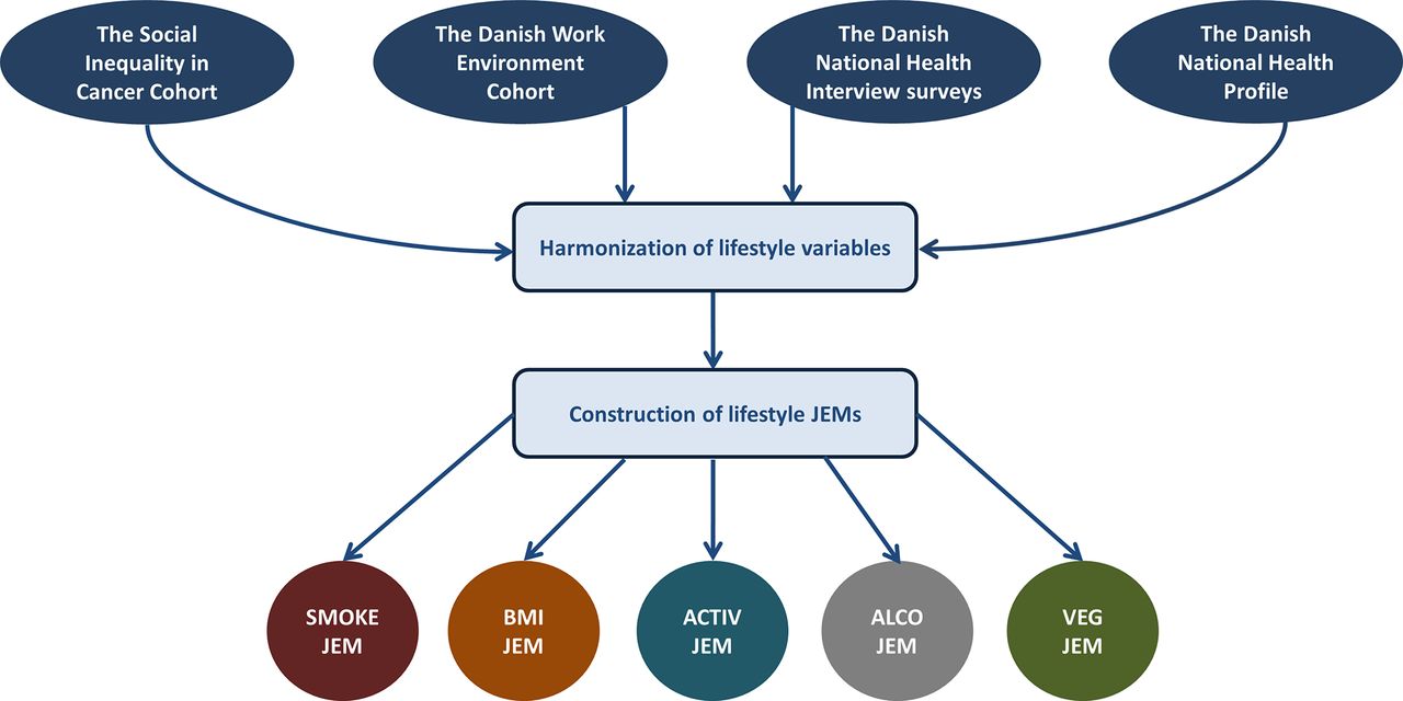
Overview of the data flow linking the respective cohort studies in one data file, where in the lifestyle job-exposure matrices(JEMs) are generated. BMI, body mass index.
Social Inequality in Cancer Cohort (SIC) comprises pooled data from seven Danish cohorts including 83 006 individuals aged 20–93 years of age at entry, primarily living in the Danish cities of Aarhus or Copenhagen. Lifestyle data were harmonised across the seven cohorts (n=76 294) as described elsewhere.13
The Danish Work Environment Cohort (DWEC) studies from the National Research Centre for Working Environment were initiated in 1990 and include nationwide random samples of employees aged 18–59.14–16
The Danish National Health Interviews (DNHI) surveys from the Danish National Institute of Public Health were carried out from 1987 through 2005. All samples were randomly drawn using the Danish Civil Registration System. Study design and characteristics of the DNHI surveys have been described elsewhere.17 18
The Danish National Health Survey (DNHS) was carried out in 2010 and 2013 at the Danish National Institute of Public Health, together with the five Danish regions. National representative surveys were conducted to provide an overview of the health, morbidity and well-being of the Danish adult population.17 19
Assessment of occupation
Individual information of occupation for all individuals in the study was available from the DOC*X database at Statistics Denmark,20 and linked to the survey data by the use of the CPR.21 In DOC*X, all employed Danish citizens are included from the age of 15, with annual information on occupational code, industry code and income. All occupational codes in DOC*X have been harmonised to the DISCO-88 classification system based on the four-digit International Standard Classification of Occupations (ISCO)-88 classification system,22 including 372 job groups. For descriptive purposes, we grouped DISCO-88 codes according to procedures from Statistic Denmark.23 24
Permission to link variables from the included cohorts and surveys with the DOC*X database was obtained from the Danish Data Protection Agency.
Assessment of lifestyle factors
Information about lifestyle factors was extracted and harmonised from questionnaire and interview data from the four data sources. We assembled a categorical variable for current smoking (0=non-smoker; 1=smoker), where ex-smokers were defined as non-smokers. Among smokers we calculated the total amount of tobacco smoked per day (gram of tobacco for each unit: cigarette=1, cheroot=3, cigar=4; pipe=3). Alcohol consumption was calculated as units of alcohol per week (12 g of alcohol in a unit). We further made a categorical variable for alcohol (0=0 units/week; 2= >0–7 units/week; 3= >7–14 units/week; 4= >14 units/week). Leisure-time physical activity was combined in one categorical variable (1=sedentary activity (≈ no sport/training); 2=low/easy waking or biking (≈ 1–2 hours/week); 3=moderate training (≈ 2–4 hours/week); 4=hard training/competitive sport (≈ >4 hours/week)). Information on height and weight was available either from questionnaires/interviews or clinical examination data for the calculating of the BMI (kg/m2). Vegetable consumption was calculated as the highest frequency of fruit or vegetables indicated in the question(s) of each data material. The frequencies were divided into three groups for frequency of total intake of fruits and vegetables per week (1=never/rarely; 2=1–6 per week; 3=daily).
Statistical methods
We restricted our study sample to men and women with an occupational code registered in the DOC*X cohort for the same year as for completion of either the questionnaire or interview.
The exposure level in a job group was calculated as best linear unbiased predictions (BLUPs) by fitting mixed models in SAS (V.9.4, SAS Institute). We used linear models (Proc Mixed procedure) except for probability of smoking, where we used mixed logistic regression (Proc Glimmix, link=logit, dist=binary). Age group (1= <30; 2=30–39; 3=40–49; 4= ≥50 years of age), gender (men/women) and source of data1–16 were included as fixed effects and DISCO-88 codes as random effect. Data were divided into 5-year intervals, except for the first 10-year interval with less participants (1=1981–1990; 2=1991–1995; 3=1996–2000; 4=2001–2005; 5=2006–2010; 6= >2010). Only job -groups with at least 10 observations were included. If <10 observations were available for a DISCO-code, the predicted value for the less detailed DISCO-code was imputed to the final JEM (eg, the predicted value for the DISCO-code 931 was imputed for the missing value of 9311). The final JEMs included predicted values for each combination of DISCO-code, gender, age group and time period. Furthermore, the number of study subjects used for the predictions and the SD for the predicted measures was included. In this article, only the results for the most detailed level of DISCO are presented.
For evaluation of each JEM on the most detailed four-digit DISCO-level, we calculated the intraclass correlation coefficient (ICC) and the highest/lowest, 95/5 and 75/5 percentile ratios for each time period. The ICC is equal to the variance between the job groups divided by the sum of the variance within and between job groups plus the residual value, and it ranges from 0 to 1 (all variation is between job groups).
We calculated Spearman correlations between JEMs to investigate any agreement between the different lifestyles.
To illustrate that the lifestyle JEMs carries independent information in addition to education, we made analyses using sex, age and the cumulated smoking at age 50 (by the smoking proportion JEM, categorised according to quartiles) as predictors, both with and without including education in Poisson regression of all-cause mortality. Education was defined as highest attained education at age 50, categorised as short (primary or secondary school or vocational), medium or long.
The population included was persons from the Danish population (employed between 1976 and 2015) with at least 20 years of (JEM-)recorded smoking exposure before the age of 50, followed -up from first employment between age 50–60 and until 2015 or death whichever came first. In total, 976 264 persons were followed for 9 458 032 years (43 326 deaths).
Results
In our study sample, 57.4% of the subjects had a job title registered in the DOC*X database for the current year, which overall resulted in a final sample of 264 054 study subjects for construction of the JEMs (table 1). Characteristics of the surveys are provided in table 2.
Distribution of gender, age and lifestyle by time period and data source
The calendar period-specific 95/5 and 75/25 percentile ratios were 1.5–2.8 and 1.6–1.9, respectively (table 3).
Crude and best linear unbiased prediction (BLUP) statistics by lifestyle factor across calendar time
Smoking
We saw a linear decline in the proportion of smokers from 56% in the period 1981–1990 to 19% after 2010 (table 3), whereas the amount of tobacco consumed by smokers only changed slightly across the years (table 3).
The predicted proportion of smokers ranged from 6% to 40% between job groups for the latest period (>2010) with a ratio between highest and lowest predicted level of 6.8, while the amount of smoking ranged from 8.0 to 19.5 g/day, corresponding to a ratio on 2.4 (figure 2).

The population distribution of the predicted values of the lifestyle job-exposure matrices across all job groups with specification of the three jobs with lowest and highest predicted values for each lifestyle JEM. 1210=directors and chief executives; 1227=production and operations department managers; 2113=chemists; 2114=geologists and geophysicists; 2141=architects, town and traffic planners; 2145=mechanical engineers; 2221=medial doctors; 224=pharmacists; 2310=college, university and higher education teaching professionals; 2419=business professionals; 3213=farming and forestry advisers; 3449=customs, tax and related government associate professionals; 3475=athletes and sportspersons; 5111=travel and attendants; 5121=housekeepers and related workers; 5123=waiters and bartenders; 5133=home based personal care workers; 5162=police officers; 5169=protective service workers; 7136=plumbers and pipe fitters; 7142=varnishes and related painters; 8141=wood processing-plant operators; 8162=steam engine and boiler operators; 8322=car, taxi and van drivers; 8323=bus and tram drivers; 83244=heavy truck and lorry drivers; 8340=ships’, deck crews and related workers; 9312=construction and maintenance labourers; 9313=building construction labourers.
The calculated ICCs for the SMOKE-JEM for proportion increased linearly from 2.7% in the first time period to 5.7% in the last, which indicates increased variability between the job groups with calendar year. Similarly the ICCs increased by time period in the SMOKE-JEM for amount of smoking (table 3).
Alcohol
Information on alcohol was available from 1981 until 2013, and no major changes in the overall intake of alcohol were observed (table 3).
Average consumption of alcoholic beverages varied between the job groups with predicted values ranging from 2.4 to 10.0 units/week (ratio=3.7) (figure 2). The calculated ICCs were small with decreased ICCs by time period from 3.80% to 1.07% (table 3).
Body mass index
In the first time period, only 23% (n=84) of the DISCO codes had BMI information at the most detailed four-digit DISCO level, whereas in the latest time period BMI information was available for 71% (n=264). The mean BMI increased almost linearly from 24.2 kg/m2 in the first time period to 25.2 kg/m2 in the latest time period (table 3). In general, men had a higher BMI than women and the BMI increased by age in all time periods. The ICCs were small with no time trend (table 3), and the predicted values ranged from 21.3 to 28.0 kg/m2 with a ratio of 1.3. Analysis of the relationship between matrix estimates for BMI and socioeconomic status indicated a positive linear relationship (R2=0.46 in >2010).
Leisure-time physical activity
Information on leisure-time physical activity was available from 1981 until 2013 but only small differences in the mean levels were found across the time periods (table 3). The level of physical activity was highest among the oldest and youngest age groups before the year 2000, but thereafter the level was lowest among the oldest age group. In general, men had a higher level of physical activity than women. The ICCs varied from 0.26% to 2.21% with no clear time trend (table 3). The predicted levels in the job groups ranged from 1.7 to 3.2 (>2010) with a ratio on 1.8.
Fruits and vegetables
Information on intake of fruits and vegetables was available from 1991 until 2013. We saw a small increase in the predicted intake during the time periods from 2.5 to 2.7 on a scale ranging from 1 to 3 (table 3). In general, women had a higher intake than men, and the intake of fruits and vegetables increased by age. The ICCs were small without any time trend (table 3). The average intake of fruits and vegetables ranged from 2.4 to 2.9 with a ratio of 1.2 in the latest time period.
Performance of the lifestyle JEMs (an example)
Most lifestyle factors are moderately correlated, though smoking and activity and BMI, and alcohol and BMI are only very weekly correlated (online supplemental table S1). The JEM-based cumulative smoking exposure is a strong predictor of death from all causes, even when simultaneously controlling for education (online supplemental table S2).
Supplemental material
Discussion
We created health behaviour JEMs based on 264 054 study subjects from different studies with interview and questionnaire data on smoking, alcohol consumption, leisure-time physical activity, BMI, and intake of fruits and vegetables. The between-job group variation was <5%–10% of the total variation, but across job groups a substantial contrast was evident with ratios between highest and lowest predicted levels ranging from 1.2 to 6.8 and with 95/5 and 75/25 percentiles ranges of 1.5–2.8 and 1.6–1.9, respectively. The analysis of all-cause mortality predicted by the smoking JEM with and without adjustment for length of education illustrates that the JEM carries substantial independent information in addition to usual lifestyle proxies as education.
Strengths and limitations
Our study is by far the biggest Danish study on lifestyle exposures measured by pooling interview and questionnaire data from several Danish surveys. The large study sample allows for estimation of lifestyle factors for about 70% of the entire workforce on a detailed DISCO level. The large time span provides time-specific estimates, which is a key issue, as lifestyle habits have changed significant in the Danish population since 1981.25 26 The lifestyle JEMs were refined by including gender, age and calendar period in the BLUP models which contributed significantly and thus served to decrease misclassification inherent in the JEM approach.
The construction of lifestyle JEMS relies in linkage of different cohort studies. Repeated cross-sectional surveys with fixed questions over time would be a useful alternative source but unfortunately no cross-sectional surveys with repeated information on both lifestyle and occupational titles are readily available.
The survey data included have used different recruitment strategies. The SIC consists of data from several cohort studies where the participants have been invited according to age group and living in defined areas of Copenhagen and Aarhus12 —the two largest cities in Denmark. The SIC data are therefore not representative for the whole country. The study populations of the DNHI, DWEC and DNHS have used other recruitment strategies, but overall with the purpose to create nationally representative samples. Overall, the number of study subjects and the representativeness increased by time period in our data, which may influence the estimated exposure values in the JEMs. The low number of jobs traditionally placed at the country side may leave us with less precise estimates for those jobs. For a given job group, however, we do not believe that the various sampling strategies introduce noteworthy bias. Participation bias may also be introduced in our estimates as a consequence of the healthy participant effect. We know from other studies that people participating in research studies in general are healthier than people who choose not to participate.27 If the healthy participant effect is introduced in our data, the predicted values for lifestyle factors may not reflect the general workforce, but only the healthiest part of it.
Another limitation in our study is that the questions used for estimation of lifestyle exposures differ between surveys. BMI is calculated in the same way for all surveys, but in the SIC cohort a large part of the measurements for weight and height is from clinical examinations. In the questionnaire surveys, weight and height are self-reported. We saw a tendency to lower BMI in self-reported data compared with data from clinical examinations, indicating that people may underestimate their weight and overestimate their height in self-administrated questionnaires. The systematic bias in BMI is supported by findings in other studies.28 29
Between-group and within-group variation
The between-group variation in health behaviours was small compared with the within-group variation as reflected in ICC values <5%–10%. This is expected because the studied unhealthy behaviours are rather prevalent regardless of type of occupation which is in contrast to rare occupational exposures.30 31 Small differences in the occurrence of unhealthy behaviours in the most prevalent occupations also contribute to small ICCs when calculations are based on the entire population. ICCs for subsets of the population defined to increase the occupational exposure contrast of interest may have substantially higher ICCs as evidenced by the ratio of unhealthy behaviour between jobs with highest and the lowest occurrence, which for some lifestyle factors proved substantial.
For smoking the ICC increased by time period, which indicated larger between-group variation by calendar year. During the 2000s, we saw major changes in the Danish Society with respect to smoking habits as educational institutions, the public transport systems, private companies, etc, began to introduce smoking policies. Furthermore, the Danish government introduced a nationwide smoking policy in 2007 with the purpose of limiting smoking at public places.32 However, this is not directly reflected in our smoking data since we saw an almost constant decline in both smoking proportion and amount of smoking from the time period 1991–1995.
For alcohol consumption, we saw the opposite pattern with decreased ICC by time period, indicating that alcohol consumption in the last decade is happening equally in all socioeconomic status groups and in all job groups, as we did not see a social gradient for alcohol consumption. For BMI, leisure-time physical activity and intake of fruits and vegetables, the ICCs were in general small and did not show a clear time-dependent pattern. This indicates that there have been no major changes in the variability between job groups for the lifestyle parameters during the time periods. However, the low ICCs could also indicate that the harmonisation of the interview and questionnaire data for leisure-time physical activity and intake of fruits and vegetables has been inappropriate to measure the variability between job groups.
How to use the JEMs
The lifestyle JEM can be used simply as a systematic and transparent external information on average health behaviours in specific jobs or—depending on the research questions—it can be applied to the entire national population or subsets of the population defined by job title to obtain the optimal trade-off between contrast of exposure and statistical power. Thus the gender, age and calendar time-specific lifestyle JEMs are intended as tools to address potential confounding in occupational register-based studies where workplace exposure assessment is assigned by JEMs. The objective was not to provide a tool for registry-based studies of lifestyle per se, but rather to enable adjustment for lifestyle in studies addressing workplace exposures where individual lifestyle information is unavailable. In addition to community-based studies, this also includes occupational cohorts with industry-specific JEMs, but without information on lifestyle. The application of lifestyle JEMs will introduce non-differential misclassification and less efficient control of confounding than use of individual data, but since the behaviour JEMs are developed for use in register-based occupational JEM studies, the misclassification of lifestyle factors is balanced to the misclassification of the exposure of interest. Hereby the lifestyle JEMs represent a systematic alternative to other methods for control for lifestyle-related confounding in occupational studies such as ad hoc adjustment of excess risk based on hypothetical assumptions about health behaviours in exposed and controls10 or use of antecedent ad hoc data on health behaviours that often are based on small samples. However, since health behaviours and lifestyle patterns are highly time-specific and country-specific the JEMs are not a priori useful in other countries.33
The estimated values for each job group can be applied to individual study subjects according to job title, gender, age and calendar time. The estimated values in the JEMs are not intended as exact exposure measures but should rather be seen as relative measures between job groups since they are not validated against external data sources. DOC*X is an open research resource, which means that researchers from all over the world can get access to the data after approval from the DOC*X steering committee, the Statistics Denmark and the Danish Data Protection Agency. More information can be found at www.doc-x.dk.
References
Footnotes
Contributors JPB, SBP and EMF conceived and designed the study. SBP and EMF analysed the data. SBP wrote the first draft which was revised by JPB. All authors contributed to the writing of the manuscript, and final version was approved by all authors.
Funding The study was funded by the Danish Working Environment Research Fund (43-2014-03/20140016763).
Competing interests None declared.
Patient consent Not required.
Provenance and peer review Not commissioned; externally peer reviewed.
Data sharing statement All data are stored at Statistics Denmark. Researcher can get online access to data, also from abroad, through contact the correspondng author who can apply for permission.