Smoothing methods with fewer assumptions about the shape of the exposure-response curve are particularly appropriate for large studies of occupationally exposed cohorts where a rising relative risk (RR) often flattens or even declines at the highest exposures.^1–4 Typically, such patterns are described either by fitting a series of parametric models with different functional forms for the dependence of risk on exposure, or by transforming exposure into a categorical variable and fitting a step function. Modelling a step function assumes uniform risk within discrete categories of exposure, but puts no constraint on the differences in risk across categories. Such a transformation, however, requires the selection of cut-points to define the categories and the selection influences the shape of the observed dose-response curve.^5–7 Moreover, even when measurement error in a continuous exposure variable is non-differential, the transformation into categories can give rise to bias away from the null^8,9 because subjects with exposure at the high (or low) end of a category, just below (or above) a cut-point, have both a greater likelihood of exposure misclassification and a higher (or lower) probability of disease than other subjects in the same exposure category. In light of these disadvantages, alternative modelling approaches are needed for occupational studies.

Spline functions are flexible statistical techniques that let the observed data determine the appropriate functional form of the dependence between exposure and response.¹⁰ There are two broad classes of splines: regression splines and smoothing splines. Regression splines are piecewise polynomials joined at distinct “knots”. The most common type of regression spline, cubic splines with linearly constrained tails, also known as restricted cubic splines, have been used to estimate hazards in survival models.^11–13 Regression splines, however, are sensitive to the location, as well as the number, of the knots. Although maximum likelihood methods can help define the knots,¹⁴ this sensitivity is reminiscent of the problem with categorising exposure described above. Alternatively, smoothing splines have knots located at every unique value of the continuous predictor variable, and include a penalty for overfitting. Smoothing splines have been used in generalised additive models (gams) to analyse environmental risk factors, such as air pollution, climate, and mortality,^15–17 and in epidemiological risk assessments of silica and lung cancer¹ and silicosis.³ In a reanalysis of a case-control study of oral cancer and alcohol consumption, both smoothing and regression splines in a logistic regression analysis suggested the absence of a threshold, a result previously obscured by a step function.¹⁸ Smoothing splines, however, are computer intensive, and may be prohibitively so in survival models for a full cohort analysis.

In 1996, a hybrid approach was developed, called penalised splines (P-splines), combining the most attractive attributes of regression and smoothing splines.¹⁹ P-splines are regression splines in which the penalty is applied directly to the coefficients of the piecewise polynomial coefficients. In this approach, one can retain a large number of knots in the regression spline formulation, but constrain their influence using the penalty term to avoid overfitting. Several authors^20–22 have shown that the resulting fit is insensitive to the precise locations of the knots as long as they are relatively “dense” enough (for example, one knot for every 3–4 unique covariate values) among the covariate observations to allow enough curvature.^20–22 The smoothness of the fit is controlled with a smoothing parameter λ, related to the severity of the constraint on the regression coefficients.

Penalised splines can be implemented using a number of different choices for the basis elements in the regression spline, including truncated polynomials, B-splines, and radial basis functions.²¹ It has been noted that for certain choices of the basis used in the regression spline, the penalised spline model corresponds to a reduced knot version of the smoothing spline, which can have large computational savings when the sample size is very large.²² This is an interesting connection, since the S-Plus function smooth.spline( ) for fitting smoothing splines also uses a low rank approximation to the full model when the sample size is large (n > 50).

In this paper, we build on our previous demonstration that P-splines can be easily incorporated into Cox regression and applied to occupational cohort data.²³ Although the relative performance of P-splines with other types of splines or smoothing methods is a subject of substantial interest, we have treated P-splines as representative of smoothing approaches and do not provide any comparisons here. Nor do we claim superiority of P-splines over other types of non-linear approaches such as fractional polynomials, which are a flexible parametric approach based on a power transformation of the data.²⁴ A formal comparison of alternative approaches would require simulation studies to evaluate model fit under different scenarios.

To illustrate the advantages of smoothing, we chose a cohort study of workers exposed to silica in the diatomaceous earth (DE) industry²⁵ because the cohort was influential in occupational health policy and because risk appeared to be a nonlinear function of exposure. This cohort contributed to the body of evidence evaluated by International Agency for Research on Cancer in its classification of crystalline silica as a human carcinogen in 1997,²⁶ and was recently the basis of two quantitative risk assessments published by researchers at the National Institute of Occupational Safety & Health (NIOSH).^1,3

In the original analysis by Checkoway and colleagues,²⁵ the rate ratio for lung cancer was modelled as a step function of cumulative silica exposure in Poisson regression. In the NIOSH reanalysis and risk assessment, Rice et al fit Cox and Poisson regression models with cumulative exposure to respirable silica treated as both a continuous and a categorical variable (with 50 levels).¹ The RR for lung cancer was modelled as a log linear, log square root, log quadratic, power, and linear function of exposure using Poisson regression. To help choose among these competing functional forms, a cubic smoothing spline (not a cubic regression spline) was used in a gam approach to examine the shape of the exposure-response relation. The best fitting model was linear up to the midpoint of the exposure range; the maximum exposure presented in the paper. There was no explanation offered in the published report for the truncated exposure range. We take the models published by Rice et al as the point of departure for this analysis, and focus on the shape of the curve over the entire range of exposure.

METHODS

Study population

The diatomaceous earth (DE) cohort includes 2342 subjects. All were white males (23% Hispanic) who were employed for at least 12 months, including at least one day between 1 January 1942 and 31 December 1987 in a DE mining and processing facility in California. Follow up covered the period from 1942 to 1994; vital status was determined for 91% of the cohort, and cause of death was ascertained for 716 of 749 (96%) deaths. There were 77 lung cancer deaths in the cohort.

Exposure

Cumulative exposure to respirable crystalline silica was based on historical reconstruction of exposures for all subjects.²⁷ The crystalline silica exposure index incorporated data on percentages of crystalline silica in the various product mixtures and secular changes in DE production at the plant. Cumulative exposure to respirable crystalline silica ranged from zero to 62.5 mg/m³-years. In the original analysis, Checkoway et al lagged exposure by 15 years and based cut-offs for exposure categories on quartiles of the total number of deaths in the cohort due to all causes.²⁵ The highest cumulative exposure category was defined to include exposures greater than 5 mg/m³-years.

In the present reanalysis exposure was treated as a continuous variable. Cumulative exposure was investigated, as were lagged cumulative exposures, constructed to account for latencies of 10, 15, or 20 years between exposure and death due to lung cancer. Lagging was accomplished by assigning zero weight to exposures in the latency period. As in a more fully parametric analysis, the amount of lagging in the final model is ultimately the investigator’s decision, based on biologic plausibility and exploratory data analysis, without clear criteria.

Confounding

For the sake of comparability with previous reports, the identical set of confounding variables was included as covariates. All regression models included: ethnicity (Hispanic yes/no); duration of follow up, to reduce healthy worker effect bias; and calendar year, to control for secular trends in lung cancer mortality during the 50 year study period. Because smoking information was only available for half the cohort and previously shown not to be correlated with silica exposure, we did not include it as a covariate.²⁵

Statistical models

We used P-splines in a Cox model, rather than Poisson regression, because it is easier to handle the time varying covariates. Risk sets were selected using SAS²⁸ to include subjects who lived to be at least the age of death of each index case and had been employed for at least one year by that age. Using S-Plus²⁹ to fit Cox proportional hazards models with P-splines, the hazard for the i-th subject in j-th stratum (case and risk set) can be written as:

where s is a smooth function of exposure X_i(t) and β_z is the vector of parameters for the other covariates, Z_i(t). A p-th degree penalised spline model for the smooth term s(X_i) is

where X_i is a particular exposure for the i-th subject, x₊  =  max (0, x), K is the number of knots, κ₁, ...κ _k are the knot locations, and p is the order, or degree, of the penalised spline. The slopes, b’s, are subject to (penalised by) the constraint:

Thus the spline curve includes additional terms as exposure increases beyond successive knots and each additional term changes the slope so that the curve has a distinct slope at each knot. The smaller B is, however, the less difference in the slopes between adjacent knots and the smoother the curve. P-splines use many knots to depict the underlying structure of the relationship, typically one knot per 3–5 observations up to a maximum of 30 to 40 knots.^20,22 An attractive feature of this approach, also shared by smoothing splines but in contrast to regression splines, is that the amount of smoothness is determined by a single parameter (B) and thus can be manipulated (via df) and evaluated more simply. (Note as B approaches 0, the p-spline approaches a polynomial function.)

The formulation (2) uses the truncated polynomial basis, which has the benefit of interpretability but can be numerically unstable in some settings.³⁰ For implementation, it is preferable to use an alternative numerically stable basis, such as B-splines¹⁹ or radial basis functions.²² As a result, the pspline function in S-Plus uses B-splines. The S-Plus code for fitting a Cox model with a penalised spline function of exposure is presented in the Appendix.

We used Akaike’s Information Criterion (AIC) to help select the optimal smoothing parameter, attentive to Hastie and Tibshirani’s caution against relying on any single criterion.¹⁰ AIC, defined as:

AIC  =  Deviance (y; μ) /n + 2df φ/n

is a measure of goodness of model fit based on the deviance with a penalty for overfitting (roughness) measured by the degrees of freedom (df). Biologic plausibility (that is, monotonicity) was considered, along with AIC, in selecting the optimal df. The default number of knots in the pspline function (S-Plus) is 2.5 times the df and they are equally placed across the range of X. We examined the sensitivity of the P-splines to the number and location of knots, for a given df. We compared P-splines implemented using the default knot selection, for example, 10 evenly spaced knots for 4 df, to those based on 30 knots placed at quantiles of the unique values of exposure. We also explored the impact of the order of the P-spline on results.

S-Plus output for P-splines includes a graphic representation of the fitted splines and standard error bars, with log hazard ratio (HR) on the Y-axis, and exposure on the X-axis. A flattened histogram, or data rug, is displayed along the X-axis. Although the density of the data is not well articulated by the rugs, regions of sparseness can be easily identified. The graphs are calibrated so that the log HR is set equal to zero at the mean exposure rather than at zero. (This has only minimal effect on the interpretation of the graphs in environmental applications because the mean exposure is generally close to zero.) In addition to the visual presentation of the fitted curve, P-splines are also described by two p values for each smoothed covariate: a p value for the linear component and a p value for the non-linear component of the curve. When penalised splines suggested a linear relation between exposure and log hazard, we used SAS (Phreg) to fit proportional hazards models with linear functions of exposure.

Model sensitivity

We examined the sensitivity of P-splines to the degrees of freedom (as well as the number and location of knots), the length of the exposure lag, and influential observations in the data. To assess the influence of the highest exposures, extreme values were trimmed and the model refit. Exposures were trimmed using two approaches: deleting the highest exposed subject(s) from all risk sets in which they appear, and deleting observations, that is, only the subject’s highest exposures, which removed the subject(s) from some, but not all, risk sets.

RESULTS

The size of risk sets for the 77 lung cancer deaths ranged from 1659 for the youngest case (age 44) to 109 for the oldest (age 80). The Cox model was based on more than 66 000 person-year observations, drawn from repeated sampling of the 2342 cohort members. On average, the lung cancer cases were hired earlier and worked slightly longer than the rest of the cohort (table 1). The average, median, and 75th centile cumulative silica exposure of the cases was more than twice that of the non-cases; however the highest exposed case had been exposed to 32.1 mg/m³-years, compared to a maximum of 62 mg/m³-years for non-cases in the rest of the cohort.

All Cox models included calendar year (at the age of the death of the index case), duration of follow up, and ethnicity, as well as cumulative silica exposure. Duration of follow up and calendar year were included as linear terms in the model. The log HR was −0.5 at zero exposure (because the curves are calibrated to be 0 at the mean exposure). Thus to interpret the curves as RR, one must add 0.5 to the observed value before exponentiation. We began the analysis using a 10 year lagged exposure, consistent with the previous study.¹

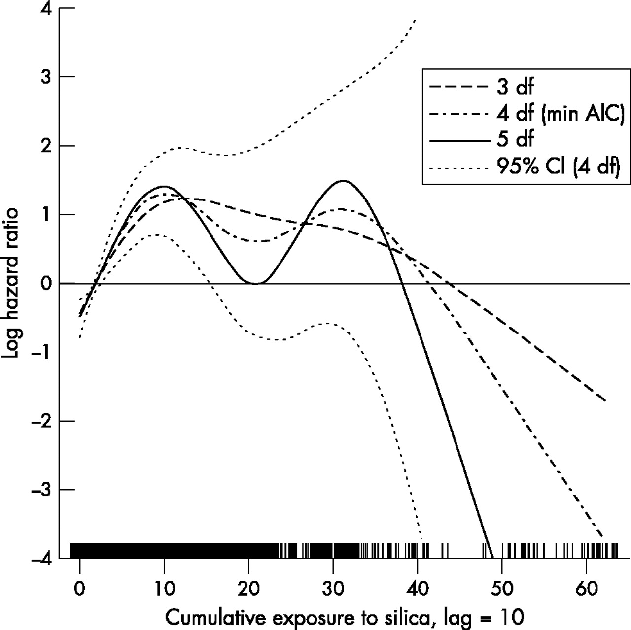
Varying degrees of freedom

The AIC was minimised when the P-splines for the smooth on cumulative silica exposure (lag 10) had 4 df. To consider alternative df, we overlaid smoothed curves with 3, 4, and 5 df (fig 1). For each curve, when we varied the order of the P-spline from 2 to 5, there were no differences in the fit of the exposure-response relations (data not shown). Thus, all the models in fig 1 were based on third order P-splines, with the number of evenly spaced knots equal to 2.5 times df. We then considered the impact of knot selection on the results. We refit the three models in fig 1 (3, 4, and 5 df) using 30 knots placed at quantiles and compared results to those based on the default knot selection. The three new curves were indistinguishable from those in fig 1 (data not shown), although the locations of the knots were dramatically different. For example, for P-splines with 4 df, the highest of the 30 knots placed at quantiles and of the 10 equally spaced knots, was 14 and 55 mg/m³-years, respectively. There was no obvious biological reason to believe the exposure-response relation was bimodal, as suggested by the curves with 4 and 5 df. Thus we judged that P-splines with 3 df were the best balance between goodness of fit and biologic plausibility.

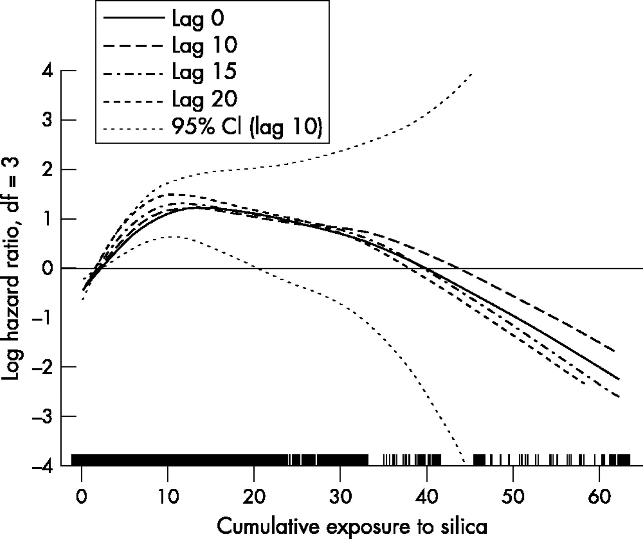
Exposure lagging

In fig 2 we present P-splines with different exposure lags (0, 10, 15, and 20 years), based on 3 degrees of freedom. All the exposure-response curves had a similar shape, with RR rising steeply at lower levels of exposure, peaking at about 10 mg/m³-years exposure, and then declining. The maximum RR increased slightly as the length of the lag increased, consistent with disease latency, and therefore supports a causal hypothesis. The difference, however, was relatively small and we have focused the subsequent analysis on the 10 year lag to allow more direct comparisons with the previously reported results.

Influence of extreme values

We relied on the visual presentation of the models to assess the influence of extreme values of exposures on the shape of the curve, over distinct regions of exposure (fig 3). The highest exposed case had a cumulative exposure of 32.1 mg/m³-years; all exposures above that belonged to non-cases. The highest exposed subject was a non-case who appeared in 72 different risk sets; with a cumulative exposure of 62.6 mg/m³-years in the last risk set. Removing this subject deleted all exposure data above 40 mg/m³-years. The second most highly exposed subject appeared in 66 risk sets. After also deleting the second non-case, exposures were truncated at 33 mg/m³-years, just above the exposure of the highest exposed case.

As seen in fig 3, deleting the first non-case did not alter the shape of the curve over the truncated range of exposure. Deleting the second most highly exposed non-case as well, however, resulted in a HR that dipped slightly and then rose to 7.4 (exp (1.5 + 0.5)) as exposure approached the maximum of 33 mg/m³-years. The 95% pointwise standard error bars based on complete data became very wide above 33 mg/m³-years, reflecting the lack of information above the highest exposed case. We also trimmed the data by removing observations rather than subjects. When we removed the observations above the exposure of the highest exposed case (32.1 mg/m³-years) the fitted curve was indistinguishable from that based on deleting the two highest exposed subjects (data not shown).

Logarithmic transformation

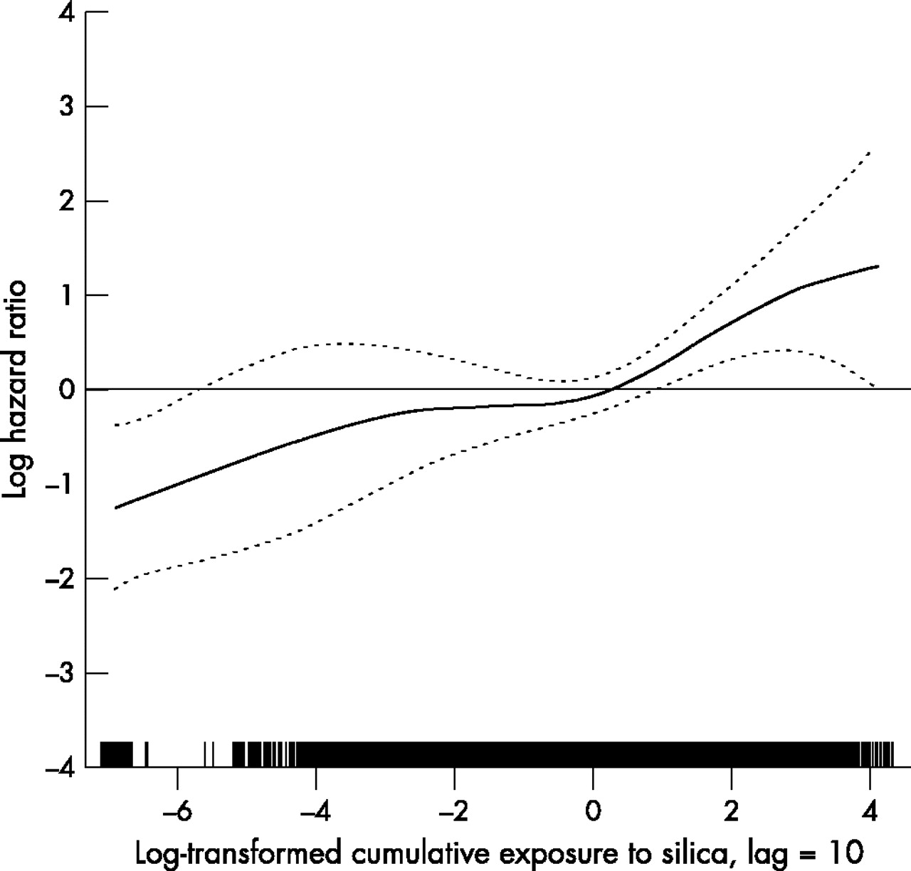
A natural log transformation of exposure was also used to reduce the influence of the highest exposed subjects and reduce skewness. To avoid taking the log of zero, we added a small constant (0.001) to each observed value of cumulative exposure. The P-spline curve (3 df) was approximately linear on the log exposure scale (p < 0.001 for the linear component and p = 0.19 for the non-linear component). To examine the sensitivity of the curve to the size of the constant, we refit the model after adding 0.01 instead of 0.001 to each exposure value. The new curve was also linear on the log-log scale, but had a wider range of exposure (data not shown). Based on the shape of the fitted P-splines in fig 4, we fit a Cox model with the log hazard as a linear function of the log transformed exposure (10 year lag). In a model adjusting for the same three potential confounders as before, the estimated HR was 1.24 per unit of log exposure (95% CI 1.11 to 1.39).

The predicted HR at given exposure levels were compared between Cox models with P-splines (fig 3) and the Cox model with a linear term for log transformed exposure (β = 0.22, se 0.06). In the lower region of exposure (below 10 mg/m³-years), the HRs predicted by the P-spline models were the same before and after excluding the two influential subjects (table 2). Except at the lowest level, however, both smoothed models yielded higher predicted RR than the log transformed linear model. The latter were quite close to the RR estimated in the original analysis to be 2.2 for all cumulative exposure greater than 5 mg/m³-years.

DISCUSSION

We have shown that P-splines are a feasible approach to modelling occupational exposure-response data in large epidemiological studies with quantitative exposure estimates. In contrast with numeric summary measures that accompany parametric models, such as regression parameters and model deviance, the visual plot of the P-spline curve provides a picture of the predicted log HR against the flattened frequency distribution (rug). If a parametric model is appropriate, the picture of how the predicted relative risk and its confidence limits behave across different regions of exposure, will point the way. In the absence of an appropriate parametric model, however, the visual presentation provides the optimal view of the exposure-response relation. Moreover, the predicted relative risks (and confidence limits) at given levels of exposure can be easily obtained from the fitted spline model (see appendix for S-Plus code).

The sensitivity of the P-spline curve to the structure of the exposure data allowed us to more fully appreciate some of the basic features of the Cox model. Risk sets defined for a full cohort analysis are nested, with subjects contained in a risk set at age t contained in all risk sets defined for ages less than t and after age of hire. Subjects who appear in multiple risk sets contribute multiple terms to the partial likelihood of the Cox model and thus have more influence on regression parameters and model fit. Such subjects may have particularly great influence if they also happen to have accumulated very high exposures. In this reanalysis, the single subject with the highest cumulative exposure to silica by the end of follow up appeared in 72 of the risk sets defined for the 77 cases of lung cancer. The visual display of splines gave a more transparent view of the exposure-response than traditional regression diagnostics for evaluating influential observations.

Residual analysis is an important tool for assessing regression model fit. But, as described by Hosmer and Lemenshow, the definition of a residual is more difficult in survival models than other epidemiological models due to censored values and the particular form of the Cox model and its partial likelihood.³² Score residuals are the primary elements of regression diagnostics for Cox models. They measure the leverage of the i-th observation on the k-th covariate as a weighted average of the distance of the value, x_ik, to the risk set means, where the weights are the change in the martingale residuals. Scaled score residuals assess the influence of individual observations on fitted Cox models by the difference in each estimated parameter before and after removing the i-th observation and refitting the model; analogous to Cook’s distance for linear regression.³³ Regression diagnostics based on observation deletion, as well as subject deletion, have recently been extended to mixed models by Fung and colleagues.³⁴ Although residuals are available in standard software packages for Cox models, they are not easy to interpret because they are not visually tied to individual subjects. We examined the scaled score residuals from a Cox model with a linear function of exposure and were able to identify the large residuals of the highest exposures. However, we were only able to assess influence of each observation by computing Cook’s distance for the single exposure parameter of the model, which in the absence of linearity is a misspecified model.

Trimming extreme values has some precedent in statistical theory. In 1962, Tukey introduced the trimmed mean as a more robust estimator of the population mean than the sample mean when the data distribution is not normal.³⁵ One possible criterion for deciding where to trim, is to define the highest exposed case as the upper end of the estimable range. Above that point we would be fitting smoothed curves in exposure regions with no cases, and would expect standard error bars around any kind of spline curves to “blow up”—that is, rapidly diverge towards positive and negative infinity. The standard error bars in figs 1–3 support the view that that the smoothed model is uninformative above the highest exposed case—that is, 32 mg/m³-years. This point was also underscored by our observation that the P-splines were extremely insensitive to the number or placement of the knots. The absence of cases in the upper half of the exposure range causes all knot parameters in this region to have large negative values, thus making the number of knots irrelevant. In this example, deleting the two highest exposed subjects was equivalent to trimming all observations greater than the exposure of the highest exposed case.

Despite precedent, there is reasonable reluctance to removing observations in the absence of a documented data error. An alternative approach for down weighting extreme values of exposures common in occupational settings is to take a log transformation of the data. In this illustration, P-splines indicated that the log HR was a linear function of the log exposure, suggesting that a Cox model with a linear term for logged exposure was also appropriate. However, the relative risks predicted by the model based on logged exposures were lower than predicted those from the spline model based on the trimmed data. It is reassuring that the differences we observed were similar to differences between the two previous analyses of these data.^1,25 Which predicted values better represent reality is an open question.

It has recently been suggested that smoothing is essentially an exploratory tool whose primary function is to point to a parametric model that fits the data well.³⁶ However, as illustrated by the difference in relative risks predicted by the spline model and the more fully parametric model identified in this reanalysis, the parametric model does not necessarily tell the same story better. We believe that penalised splines can also provide an exposure-response curve useful for aetiological research as well as for public health intervention and therefore should be presented alongside any more parametric option to provide a more complete characterisation. To make these methods more accessible, S-Plus code is presented in the appendix.

APPENDIX

The S-Plus code for fitting a Cox model with a penalised spline function to the lung cancer data in the silica cohort is presented below. The explanatory variables in the Cox model include continuous variables for cumulative exposure to silica with 10 years lag (CRISLG10), calendar time of death or risk age (CALTIME), and duration of follow up (FOLLOWUP), as well as a dummy variable for Hispanic ethnicity (HISP) with two levels. In the model specified below, P-splines are used to smooth exposure and both calendar time and length of follow up are modelled as linear terms, each with a single parameter.

The function coxph in S-Plus fits a Cox PH model, while the pspline function fits the P-spline function with N degrees of freedom, denoted by df = N. The time variable is age denoted by the variable CASEAGE, while the censoring variable is CASE, set equal to 1 for cases and 0 for non-cases in the risk sets. Risk sets are constructed based on age and denoted by the variable STRAT. Ties are handled by a command: method = “breslow”, a character string that needs to be specified (default is Efron). The function “na.action” is a missing-data filter function. In the beginning, a temporary name, cox.temp, is assigned to the dataset lungcanc to protect original data.

cox.temp<-lungcanc

coxout <−coxph(Surv(CASEAGE,CASE)∼ pspline(CRISLG10, df  =  N) + HISP + CALTIME + FOLLOWUP + strata(STRAT), data = lungcanc, na.action = na.omit, method = “breslow”)

print(coxout)

The following S-Plus code saves the fitted values and standard errors of the P-spline for exposure variable (CRISLG10) and then plots the fitted values and confidence bands of the P-spline along with the data rug [S-Plus 2000 Guide to Statistics, Volume 2″, May 1999, MathSoft, Data Analysis Products Division, MathSoft, Inc., Seattle, Washington].

tpos <−1

temp <− predict(coxout, type = “terms”, se.fit = T)

tfit <− temp$fit[,tpos]

sfit <− temp$se.fit[,tpos]

tlower <− tfit −1.96*sfit

tupper <− tfit +1.96*sfit

fit.se <− cbind(tfit, tlower, tupper)

jj <− match(sort(unique(cox.temp[,“CRISLG10”])), cox.temp[,“CRISLG10”])

matplot(cox.temp[jj, “ CRISLG10”], fit.se[jj,], type = “l”, lty = c(1,2,2),

xlab = “Cumulative Exposure to Silica, Lag = 10”, ylab = “Log Hazard Ratio, df = 3”)

rug(jitter(CRISLG10))