Article Text

Abstract
Study objective: To assess the short term association between air pollution and mortality in different zones of an industrial city. An intra-urban study design is used to test the hypothesis that socioeconomic characteristics modify the acute health effects of ambient air pollution exposure.
Design: The City of Hamilton, Canada, was divided into five zones based on proximity to fixed site air pollution monitors. Within each zone, daily counts of non-trauma mortality and air pollution estimates were combined. Generalised linear models (GLMs) were used to test mortality associations with sulphur dioxide (SO2) and with particulate air pollution measured by the coefficient of haze (CoH).
Main results: Increased mortality was associated with air pollution exposure in a citywide model and in intra-urban zones with lower socioeconomic characteristics. Low educational attainment and high manufacturing employment in the zones significantly and positively modified the acute mortality effects of air pollution exposure.
Discussion: Three possible explanations are proposed for the observed effect modification by education and manufacturing: (1) those in manufacturing receive higher workplace exposures that combine with ambient exposures to produce larger health effects; (2) persons with lower education are less mobile and experience less exposure measurement error, which reduces bias toward the null; or (3) manufacturing and education proxy for many social variables representing material deprivation, and poor material conditions increase susceptibility to health risks from air pollution.
- GLM, generalised linear model
- CoH, coefficient of haze
- SO2, sulphur dioxide
- NT, non-trauma
- AIC, Akaike information criterion
- CT, census tract
- MPC, mean percentage change
- air pollution
- mortality
- acute effects
- socioeconomic factors
- GIS
Statistics from Altmetric.com
- GLM, generalised linear model
- CoH, coefficient of haze
- SO2, sulphur dioxide
- NT, non-trauma
- AIC, Akaike information criterion
- CT, census tract
- MPC, mean percentage change
Many time series studies have reported significant, positive associations between short term ambient air pollution exposure and daily mortality,1–17 but the question of whether socioeconomic characteristics modify the acute health effects of air pollution remains unanswered. One study from Sao Paulo, Brazil,10 found that persons in districts with higher socioeconomic characteristics were slightly more susceptible to air pollution effects than those with lower ones. Yet, given the comparatively low incomes in Brazil, questions persist about whether this result would extend to wealthier countries. Another study on 20 US cities suggested no significant effect modification by socioeconomic characteristics, although this analysis was conducted at the county scale, which may not capture underlying socioeconomic gradients that tend to vary by neighbourhoods.18 Two other time series studies indicated significant effect modification by educational status measured at the individual level, with persons of lower education experiencing larger effects.19,20 The limited number of studies and conflicting results highlight a need for more research on whether socioeconomic characteristics modify the acute health effects of air pollution. Increased knowledge on socioeconomic effect modification may lead to enhanced understanding of an environment-health relation thought to have large population health impacts.5
In this paper we assess the short term association between air pollution and mortality in different zones of Hamilton, Canada. Hamilton is an industrial city located at the western end of Lake Ontario, about 60 km from Toronto. We use an intra-urban study design to test the hypothesis that socioeconomic characteristics modify the acute health effects of ambient air pollution exposure.
METHODS
Study site description
The city of Hamilton (population about 320 000) offers a “natural experiment” for testing associations between intra-urban air pollution exposure and mortality for five reasons. Firstly, the city houses one of the largest steel making complexes in North America, producing spatially concentrated pollution emissions in the north east end near the industrial core. Secondly, the circulation of cool north east breezes off Lake Ontario and the presence of the 100–120 metre high Niagara Escarpment above Lake Ontario, 3 to 4 km from its shore, combine to produce advective temperature inversions that disperse pollution from the steel mills along the lakeshore toward large and densely populated portions of the city below the Escarpment.21,22 These inversions create gradients of pollution that run from high in the north east to low in the south, west, and some parts of the east end of the city.23,24 Thirdly, the city has increased potential for environmental injustice, with lower socioeconomic neighbourhoods concentrated in high pollution areas.25 Fourthly, the presence of industry has prompted government monitoring at the intra-urban scale. Finally, the geographical extent of the city is about 24.5×12 km, providing adequate exposure contrast for intra-urban analysis.
For this study, we divided Hamilton into five zones based on Thiessen polygons that used government pollution monitors as the central nodal point. Thiessen polygons have the property that all points within the polygon are closer to the nodal point (that is, the monitoring site) than to any other site.26 This research design allows for subsequent testing of socioeconomic effect modification, while minimising the potential for exposure misclassification. Because time activity studies indicate Canadians spend about 67% of their time at home,27 we expect monitors within the zone to supply a stronger correlation with personal data than with a central monitor. We recognise this assertion is still open to debate based on the results of some personal monitoring studies28,29 and mathematical exposure models.30 Most of the personal monitoring studies, however, rely on limited samples of susceptible individuals, who may not be representative of the socio-spatial range,31 or they measure PM2.5 or sulphates,32 which are probably the most spatially homogeneous constituents of the intra-urban pollution mixture.
Data
Within each zone, we assembled daily counts of non-trauma (NT) mortality and pollution concentrations. Mortality data from the registrar general of Ontario covered the period 1985–94. These data were linked to place of residence at the time of death through the Statistics Canada 1998 postal code conversion file.33 We assigned individual mortality data to the zones through a point in polygon overlay with Arcview 3.2 Geographic Information System (GIS) software (ArcView GIS, Redlands, CA, 1999).
Two pollutants were used for the analysis: PM as measured by the coefficient of haze (CoH) and sulphur dioxide (SO2). Data on these pollutants were supplied by the Ontario Ministry of the Environment. We attempted to assemble data on other pollutants such as NO2, but found only CoH and SO2 had a sufficient number of monitoring stations for the period when we could obtain enough mortality data in each zone to conduct separate analyses. Figure 1 illustrates the zones used for analysis; the total deaths over eight and nine year periods, respectively, for SO2 and CoH data; and the average ambient concentrations of CoH and SO2 for the periods of study (SO2 was only available from 1987 on). Mortality counts range from 4267 to 6763 per zone. Table 1 shows the descriptive statistics for mortality and air pollution in the city and the zones.
Descriptive statistics for pollution and mortality data
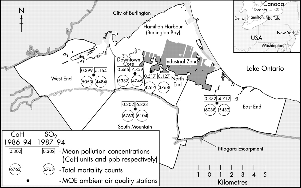
Study area with average 1986–94 coefficient of haze, 1987–94 sulphur dioxide, and corresponding mortality counts in the Thiessen polygon zones.
SO2 was measured with a spectroscopic technique based on the principle of fluorescence.34 CoH measures suspended particles continuously by paper tape sampler with an inlet flow regulated to favour small airborne particles.35 Published research supports the use of CoH as an indicator of PM in health studies (for example references9,13,36–40). We computed daily averages of each pollutant for days with 18 or more hours of complete data.
Meteorological data used for developing weather models that control for confounding of the air pollution-mortality association by coincident weather patterns were collected at the Hamilton Airport weather station operated by the Meteorological Service of Canada (MSC). Social, economic, and demographic data were extracted from the 1991 census of Canada.
Statistical models
Serial autocorrelation in the mortality data was filtered using natural splines with degrees of freedom based on the Bartlett test for white noise. The weather model relied on three variables found to be significant predictors of mortality in past Canadian air pollution studies (relative humidity, maximum temperature, and maximum change in barometric pressure at 0 to 3 day lags).1,3,4,16,41 A manual forward selection was also implemented to derive the final weather model.
After selecting the weather model based on the Akaike information criterion (AIC), it was incorporated into a larger generalised linear model (GLM) with a Poisson link. This model used mortality counts as the response variable and the natural spline of the Julian day and weather variables, a day of the week mortality factor variable, and air pollution as predictor variables. Models were implemented in S-Plus 2000 software (S-Plus for Windows, Seattle, WA) with a stringent convergence criterion (that is, 10E-14).42
Aggregate models were run for the entire city using regional average estimates of pollution from all five monitors and total NT mortality counts. These estimates were used as a baseline against which zonal estimates were compared. Separate models were run in each of the five zones. The specific model formulation of the model is given below:

i indicates the day in the time series and Yi is the number of deaths on day i.
We conducted sensitivity analyses with separate weather models and mortality smoothers for each zone. Sensitivity analyses were also undertaken based on alternative weather models with a larger set of 24 weather variables. Because the results were robust to locally optimised models and alternative weather models, we report only the results using the above specification to allow for easy comparison among the risk estimates. A final sensitivity analysis entailed combining the zones with similar social characteristics. Results of this analysis are explained in the next section.
To test for heterogeneity among the estimates, we implemented a maximum likelihood random effects model.43 This model estimates a pooled effect and tests for differences between the estimates derived for the individual zones and the entire city.
We calculated social, economic, demographic, and lifestyle characteristics for the zones to assess potential effect modification through a point in polygon overlay that included the centroids of the census tracts (CTs) contained in the pollution zones. Smoking rates for each zone were derived from previous random surveys.44 We also generated new variables measuring the average distance of the CT centroids to the nearest hospital with ArcView 3.2 and mean age of death in each zone from our mortality data (see table 2 for descriptive characteristics).
Social, economic, and demographic characteristics of the city and zones
Finally we regressed the mean percentage change (MPC) in mortality associated with pollution exposure from the largest multi-day lag onto the socioeconomic characteristics of each zone and of the regional estimate (MPC = [RR−1]×100). In this analysis we used lag123 (that is, daily pollution values averaged one to three days before death). These models were plotted for visual inspection and weighted by the inverse of the variance on the estimates. When the theta heterogeneity parameter from the random effects model was positive, the weight equalled the inverse of the variance plus θ.
RESULTS
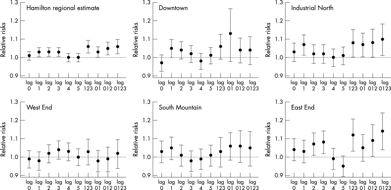
The results of the models using common smoothing spans and weather models are summarised in figures 2 and 3. These figures illustrate the relative risk (RR) and 95% confidence intervals of mortality based on the regional mean value of each pollutant compared with no pollution. Full results for models using both the regional mean of pollution and the zonal means are given in the appendix (see journal web site http://www.jech.com/supplemental). Risk estimates using the local pollution means are similar to those with the regional mean, although the size of the effects tends to be attenuated in the east end.

Comparison of regional and zonal relative risks of mortality evaluated at the regional mean of coefficient of haze.

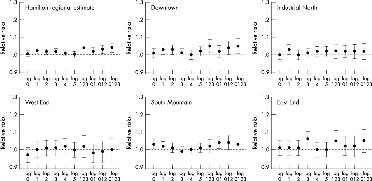
Comparison of regional and zonal relative risks of mortality evaluated at the regional mean of sulphur dioxide.
In the regional models, both CoH and SO2 have significant, positive associations with mortality. Pollution effects for the most significant individual lags (1,2,3) in the CoH models have a RR of 1.03 when evaluated at the regional mean of pollution. The multi-day lag effects for Lag123 and Lag0123 are around 1.06. The estimate for Lag012 is about 1.05. For SO2 regional models, the effects are smaller, with a 1.02 RR for single day lags (1,2,3) and 1.04 for Lag123 and Lag0123, while Lag012 is about 1.03. In general, temporal patterns in the risks follow what we would expect with larger effects at lags 1–3 and insignificant effects for lags 4–5.
For the zonal CoH models, only the downtown, the industrial north, and the east end zones show significant effects. The south mountain and west end display no significant effects at any lag in these models. The most significant one day lags for CoH in the three zones range from 1.05–1.08, or about 1.7–2.7 times greater than those for the regional models. The largest single day lag is in the east end (Lag3), followed by Lag1 in the industrial north, then Lag1 in the downtown core. Multi-day lags from the zones range from 1.06–1.14, or one third to 2.3 times higher than the regional estimate.
The SO2 results for the zonal models also display intra-urban heterogeneity, although the results are less pronounced than in the CoH models. With the SO2 models, only three zones display significant effects: east end, south mountain, and the downtown. In the downtown, Lag1 and Lag2 each have a RR of about 1.03, roughly one half greater than in the regional model. Multi-day lags in this zone have RRs of about 1.05 for both Lag123 and Lag0123. Lag012 has a smaller effect (RR~1.04). In the east end, only Lag3 shows a significant effect, but it is quite large (RR = 1.06), three times greater than in any single day lag in the regional models. One major difference in the pattern relates to the SO2 effect on the south mountain. Unlike the CoH models, this zone has a significant effect at Lag0 (RR = 1.03). Multi-day models for Lag01 and Lag012 also produce a RR of 1.04. As with the CoH models, SO2 had no significant effect in the west end.
We also ran co-pollutant models for the largest and most significant lag across the city and each zone. Only the industrial north produced a significant lag for SO2 in the co-pollutant models (see appendix for results from all zones).
Although some of the zones appear to have large differences in the risk estimates, the random effects model revealed these to be insignificant (table 3). The θ value representing the random effect for the CoH models at Lag1 indicates some heterogeneity exists among the estimates, but no more than would be expected by chance. For the CoH models at Lag123 and SO2 with both single and multi-day lags, the θ value is negative, indicating any observed variability results from sampling error. Pooled estimates derived from combining the effects nearly equal those derived from the regional model.
Comparison of regional analysis (RA) to pooled random effect (RE) models
We implemented another sensitivity analysis by combining the west end and south mountain zones into one zone. The remaining three zones (east end, north east end, and downtown) were also combined. The results are shown on tables 4 and 5. In general we see the higher status zone has effects that are insignificant, but at Lag0123 significant effects exist for both CoH and SO2; these effects are slightly higher than the regional estimate. For the lower status zone, we see effects that are significant for single and multi-day lags. These are also higher than the regional estimate, but less so than those in some of the smaller zones. Overall, the effects are smaller and less significant in the zones with higher socioeconomic characteristics than in zones of lower status.
Results from sensitivity analysis of combined high socioeconomic zones (west and south mountain)
Results from sensitivity analysis of combined low socioeconomic zones (downtown, north east, and east)
Plots of the MPC in mortality on socioeconomic characteristics in the zones appear in figures 4 and 5. A few zonal characteristics have significant associations with the CoH pollution effect: manufacturing employment and educational attainment, each with r2 values around 62%. Other models were suggestive of relations, particularly smoking and mean age of death, although these had insignificant regression coefficients due probably to larger variances on the weights and the small number of observations. Table 6 presents the correlations among the zonal characteristics. This table indicates that while only a few of the socioeconomic variables achieved formal significance, many of the variables relate closely to each other.
Zero order correlations among social, economic, and demographic characteristics for the zones

Mean percentage change in mortality from the coefficient of haze models regressed on socioeconomic, demographic, and lifestyle variables.

Mean percentage change in mortality from the sulphur dioxide models regressed on socioeconomic, demographic, and lifestyle variables.
DISCUSSION
For both the pollutants tested, significant effects were found at the regional level. Zonal estimates were from one third to three times higher than the regional model for both pollutants. The west end with the highest socioeconomic characteristics displayed no significant effect in any of the models, while the east end—a zone with low educational status and high manufacturing employment—had the largest effects. Random effects tests revealed no significant difference between the zonal and regional estimates, but weighted regression analyses suggested underlying socioeconomic characteristics modify the health effects of air pollution exposure.
The positive association of manufacturing employment and the size of the pollution effect may signal that higher total exposure to airborne particles exerts a larger effect on health. The preponderance of employment in the steel industry—known to have high occupational exposures of toxic substances,45 combined with ambient pollution—may lead to a higher dose and subsequent response. Manufacturing workers may also carry toxic substances into the home, leading to “para-occupational” exposures. This finding suggests that future research needs to examine total personal exposure in groups likely to experience high occupational exposures.
Alternatively, education, and manufacturing employment may represent a complex of variables related to material deprivation. Education generally relates to income levels, which in turn correlate to residential environment and access to medical care.46 Interestingly, geographical medical care is inversely related to socioeconomic characteristics here, but the east end zone with the largest distances still has the largest health effects. Higher education and associated income may also increase the use of air conditioning in the home, which would reduce indoor exposures.47
The sparse number of zones and complexity of socioeconomic characteristics limits our ability to draw conclusions about which specific socioeconomic variable modifies the air pollution effect. Table 6 illustrates the strong correlations between education, manufacturing, smoking, household income, and unemployment. Recent research in smaller areas of Hamilton infers that many of the socioeconomic variables in this analysis may be better represented through underlying principal components that capture complex interrelations among socioeconomic indicators.18 We were prevented from pursuing this strategy because of the limited number of zones.
Key points
-
This paper addresses the question of whether socioeconomic characteristics modify the acute health effects of ambient air pollution exposure
-
Significant health effects were associated with ambient air pollution exposure in a citywide model and in intra-urban zones with lower socioeconomic characteristics
-
Educational attainment and manufacturing employment in the zones significantly and positively modified the acute health effects of air pollution
-
Further research is needed to assess whether similar effect modification occurs elsewhere and to understand why effect modification follows socioeconomic gradients
Policy implications
-
Modification of air pollution health effects by socioeconomic characteristics could have important policy implications
-
Our results show that the largest health effects from ambient air pollution exposure occur in areas with lower socioeconomic characteristics
-
If groups with lower socioeconomic characteristics are disproportionately affected by air pollution, governments may have to target pollution control policies to reduce pollution proportionately more in areas with low socioeconomic characteristics
-
We see two obstacles to implementing such targeted policies: (1) groups with lower socioeconomic characteristics often have less political power with which to influence the policy agenda; and (2) targeted interventions will complicate implementation of air pollution control policies, which may be unpopular with regulators
-
As an interim measure, government regulators could pursue “softer” educational and subsidy policies to encourage reductions in indoor air pollution exposure for areas with lower socioeconomic characteristics
Another interpretation would emphasise intra-urban differences in the constituents of pollution. Areas observed to have larger health effects (downtown, north, and east ends) may have higher toxic emissions from point sources or more damaging particles because of higher toxic constituents. Moreover, exposure misclassification may still affect the results because the government monitoring sites represent different types of exposure. The north end monitor, for example, is known as a compliance monitor, intended primary to enforce environmental regulations at the “point of impingement” into residential areas. By contrast, the east end monitor is located in a residential area.
Intra-urban mobility may also confound the exposure assessment. Persons with lower socioeconomic characteristics may be less mobile than those with higher position.48 Less mobile persons may experience lower exposure measurement error than those with higher mobility. In this instance, we would expect areas with less measurement error to produce larger effects,49 and by extension, areas of lower socioeconomic characteristics may experience larger health effects. Future research may investigate issues of intra-urban monitoring location, toxicity, and mobility in relation to exposure measurement error.
The uniqueness of the Hamilton study site raises questions of external validity about our findings. Hamilton was chosen as a site that afforded social and environmental gradients. Individual level data on socioeconomic characteristics or pooled analysis from numerous cities would advance the research agenda even further than single city analyses. While our results remain tentative because of inherent limits in the study site, they contribute to a growing literature suggesting that socioeconomic position modifies the health effects of air pollution. The key question for future research rests in explaining why, among various competing hypotheses, socioeconomic characteristics may modify the health effects of ambient air pollution exposure.
Acknowledgments
We acknowledge funding from the Toxic Substances Research Initiative, a granting programme administered jointly by Health Canada and Environment Canada. We also thank Dr Malcolm Sears, McMaster University, for sharing his data on smoking prevalence with us. Mr Ric Hamilton and Mr Patrick De Luca, McMaster University, helped to prepare the figures and maps. Finally, we thank four anonymous reviewers and the editor for comments that improved the paper.
REFERENCES
Supplementary materials
. Web-only Appendix
Full results for models using both the regional mean of pollution and the zonal means.
Table A1 Full results for the downtown zone: estimated at the local mean of pollution
Table A2 Results for the industrial zone: estimated at the local mean of pollution
Table A3 Results for the east end zone: estimated at the local mean of pollution
Table A4 Results for the south mountain zone: estimated at the local mean of pollution
Table A5 Results for the west end zone: estimated at the local mean of pollutionThis appendix is available as a downloadable PDF (printer friendly file).
If you do not have Adobe Reader installed on your computer,
you can download this free-of-charge, please Click hereFiles in this Data Supplement: