Article Text

Abstract
Objectives Beryllium has been identified as a human carcinogen on the basis of animal and epidemiological studies. The authors recently reported updated associations between lung cancer and beryllium exposure in a large, pooled occupational cohort. The authors conducted the present study to evaluate the shape of exposure–response associations between different exposure metrics and lung cancer in this cohort, considering potential confounders (race, plant, professional and short-term work status, and exposure to other lung carcinogens).
Methods The authors conducted Cox proportional hazards regression analyses of lung cancer risk with cumulative, mean and maximum ‘daily weighted average’ (DWA) exposure among 5436 workers, using age-based risk sets. Different exposure–response curves were fitted to the exposure metrics, including categorical, power, restricted cubic spline and piecewise log-linear fits.
Results The authors found significant positive associations between lung cancer and mean (p<0.0001) and maximum (p<0.0001) exposure, adjusting for age, birth cohort and plant, and for cumulative (p=0.0017) beryllium exposure, adjusting for these factors plus short-term work status and exposure to asbestos. The best-fitting models were generally categorical or piecewise log-linear, with the steepest increase in lung cancer risk between 0 and 10 μg/m3 for both mean and maximum DWA exposure and between 0 and 200 μg/m3-days for cumulative DWA exposure. The estimated mean DWA beryllium exposure associated with 10−3 excess lifetime risk based on the piecewise log-linear model is 0.033 μg/m3.
Conclusion This study provides evidence that lung cancer risk is elevated at levels near the current US Occupational Safety and Health Administration beryllium exposure limit of 2.0 μg/m3 DWA for workers.
- Occupational
- epidemiology
- lung cancer
- metals
- density sampling
- cancer
- mathematical models
Statistics from Altmetric.com
What this paper adds
Beryllium has been designated a known human carcinogen based upon human and animal studies of lung cancer, including recent follow-up of a cohort of US beryllium-processing workers.
This study finds strong quantitative associations between lung cancer and cumulative, mean and maximum beryllium exposure, after adjusting for confounding.
Quantitative risk assessment suggests that lung cancer risk may be excessive at current occupational exposure limits.
Beryllium exposure has long been associated with an immune-mediated, granulomatous lung disease termed chronic beryllium disease.1 Toxicological and epidemiological studies have more recently led the International Agency for Research on Cancer to designate beryllium as a human carcinogen.2 3 Epidemiological evidence for the carcinogenicity of beryllium derives largely from studies within a pooled cohort of male workers4 5 at seven US beryllium processing plants, and a nested case–control study of lung cancer at one of the plants.6 7 We recently reported updated associations between cumulative and maximum beryllium exposure and several diseases of a priori interest (including lung cancer), within a three-plant subcohort having detailed beryllium exposure data.5 Although smoking data were available for only a subset (25%) of cohort members, the positive exposure–response associations observed in that study showed little evidence of confounding by smoking, as measured by indirect methods.
The present study was conducted to evaluate the association of mean, maximum and cumulative beryllium exposure with lung cancer mortality, considering potential confounders, including age, race, birth cohort, exposure to other lung carcinogens, short-term employment (workers exposed to high levels may have left the workforce due to adverse acute reactions) and professional work status (as a surrogate for smoking6). We also explored the fit of alternative exposure–response curves using restricted cubic spline models,8 followed by consideration of good-fitting categorical, power and piecewise log-linear models. Finally, we used good-fitting exposure–response models to estimate the lifetime excess absolute risk of lung cancer mortality associated with mean beryllium exposures at the current recommended exposure limit (0.5 μg/m3 as a time-weighted average) of the National Institute for Occupational Safety and Health (NIOSH)9 and to estimate the mean exposure levels associated with 10−3 lifetime excess absolute risk.
Methods
Cohort description and follow-up
The cohort consists of 5436 male workers employed for at least 2 days at one of three beryllium-processing plants, in Elmore, Ohio, Hazleton, Pennsylvania, and Reading, Pennsylvania, before 1970. These facilities were selected from the seven plants in the pooled cohort because they have substantial historical exposure data and detailed work history information for each worker, permitting the development of job-exposure matrices (JEMs). Cohort assembly and follow-up are described elsewhere.4 5 Briefly, vital status and causes of death were ascertained to 31 December 2005. Workers were considered lost to follow-up if they were last observed before 1 January 1979, the start of the US National Death Index (NDI). Follow-up for each worker began on the third day of employment and ended on the earliest of the date of death, the date lost to follow-up or the end of the study (31 December 2005).
Risk set creation
Lung cancer cases were identified from death certificates or NDI-Plus, using the following International Classification of Diseases (ICD) codes, for the revision in effect at the time of death: ICD codes 047.B-047.F in ICD-5; 162–163 in ICD-6; 162–163, excluding 162.2, in ICD-7; 162 in ICD-8 and -9; C33–C34 in ICD-10. For each lung cancer case, an age-based risk set was selected.10 Cases were permitted to serve as risk set members for other cases (provided they met the above criteria). Exposure for each risk set member was truncated at the case age at death, minus any lag. Risk sets so selected have been demonstrated to be properly matched on attained age,10 11 even when using an exposure lag.12 To permit the greatest analytical flexibility, no other factors were matched, and the full risk set was used for all statistical analyses.
Exposure assessment
The creation of JEMs for the Reading, Hazleton, and Elmore plants is described elsewhere.13–15 In brief summary, plant personnel measured exposure for a wide range of plant departments and operations, using consistent methods across facilities and time periods, and compiled exposure data on a quarterly basis. The available data were in the form of ‘daily weighted average’ (DWA) exposures (a form of time-weighted average). DWAs were computed by collecting short-term samples (both general area and personal breathing zone), measuring beryllium exposures for different tasks across a daily work shift, and calculating the time-averaged exposure concentration (in μg/m3) by multiplying the concentration by the time spent in the task, summing over all tasks and dividing by the total time in the shift. In developing the JEM, annual DWA exposures were calculated for each job and department combination using the geometric mean of the quarterly DWAs. Workers were assigned time-dependent exposures from the JEM by job, department and year (described in more detail in Schubauer-Berigan et al5). Professional judgement of two or more industrial hygienists was used to determine whether the job–department–year combination involved potential exposure to other known lung carcinogens (acid mist, asbestos, cadmium, chromium, nickel and silica).
Cumulative exposure (in μg/m3-days) was the sum of the daily average exposures (multiplied by 5/7 to permit assumption of a 5-day workweek) from first exposure to the cut-off date, minus any lag. The mean exposure (in μg/m3) was calculated by summing the DWA (not multiplied by 5/7) from first exposure to the cut-off date (minus any lag), divided by the number of days in the interval. Maximum exposure (in μg/m3) was calculated as the highest annual DWA (not multiplied by 5/7) for the worker from the start of exposure to the cut-off date (minus any lag).
Each other lung carcinogen listed above was treated as a fixed binary (ever/never exposed) covariate, based on information from the JEM. Professional worker status (a surrogate for likely smoking behaviour or exposure to other occupational lung carcinogens) was as defined previously.6 13 Short-term work status was defined as having worked less than 1 year at one of the beryllium facilities and was included to account for dropout from the workforce of high-exposed individuals who had adverse skin or respiratory reactions to beryllium.5 In considering plant as a confounder (the Reading plant had the highest beryllium exposure but was in a county with the lowest background lung cancer risk), workers employed at both Hazleton and Reading (n=30) were assigned to the plant of longest employment.
Statistical analyses
Risk sets were analysed using conditional logistic regression with age as the timescale, using the PHREG procedure in SAS (ver. 9.2). Partial likelihoods so produced, when the full risk set is used, are identical to those from Cox proportional hazards regression. Hazard ratios (HRs) for lung cancer mortality were estimated for cumulative, mean and maximum DWA exposure. Indicator variables were used for all categorical variables. All analyses are age-adjusted by the matched design and were further adjusted for birth year in categories of <1900, 1900–1919, 1920–1929 and ≥1930. These categories were selected based on predicted background risk due to birth cohort-specific smoking rates, which has been shown to be an important confounder at one plant in this cohort.7 Increasing the number of birth cohort categories, using restricted cubic splines to fit birth cohort effects, or varying the cutpoints changed the results little (data not shown). Adjustment was evaluated for the following potential confounders not on the causal pathway between beryllium exposure and lung cancer: race (white or all other races combined), plant, professional work and short-term work status, and exposure to acid mist, asbestos, cadmium, chromium, nickel and silica. A change in the HR for the beryllium metric of >10% for categorical or power models was used to select the final model for further analyses. Interactions for birth cohort, race, time since last exposure, professional work status, short-term work status, plant and potential asbestos exposure were evaluated using the product of each with each beryllium exposure metric, and conducting a likelihood ratio test of the significance of the additional interaction terms. Final models were checked for proportionality of hazards with age by evaluating its product with each exposure metric as an interaction term in the model.
For categorical analyses of cumulative and maximum DWA exposures, approximate quartiles of the case distribution were used to select cutpoints (560, 2600 and 10 000 μg/m3-days for cumulative and 4.1, 24 and 60 μg/m3 for maximum exposure), as is common in categorical analyses.16 For mean exposure, approximate quintiles of the case distribution (with cutpoints at 2, 8, 16 and 35 μg/m3) were used to permit better evaluation of low-exposure associations. In supplemental analyses for mean exposure, we evaluated the effect of choice of cutpoints on estimated lung cancer risks by fitting five-category models with different sets of cutpoints. The Akaike Information Criterion (AIC) was used to select the best-fitting categorical model.17
Initial analyses using continuous exposure–response models were based on power models (ie, log-linear models using a log-transformed exposure variable). This transformation was suggested by previous studies within this cohort,5–7 and has been used in exposure–response modelling for silica and lung cancer.18 For power model analyses, small values were added to avoid taking the log of zero for workers whose exposure was zero in lagged analyses.19 For mean and maximum DWA exposure, 0.05 μg/m3 (half the detection limit before 1996) was added for each worker. For cumulative exposure, 0.05 μg/m3-days (half the lowest non-zero exposure value in the risk sets) was added. Previous analyses within one of the cohorts included here7 showed that the choice of small value made little difference in the point estimates or p values. To verify this in the current study, additional analyses were conducted, adding half the lowest exposure value (0.0009 μg/m3 and 0.02 μg/m3 for mean and maximum DWA exposure, respectively).
To evaluate statistical significance, two-sided 95% CIs were calculated using either Wald-type methods (β±1.96×SE(β)) or profile likelihood methods. Exact p values are reported for some analyses. All primary exposure–response analyses were conducted using a 10-year lag, based on a priori considerations and earlier findings within one of these cohorts.6 7 Alternative lags (0, 5, 15 and 20 years) were also evaluated using the final models, and the lag producing the lowest AIC was considered the best-fitting model.
To assess empirically the shape of the exposure–response curve, three-, four-, five-, six- and seven-knot restricted cubic spline models were fitted to the three untransformed exposure metrics.8 17 The knots were chosen based on percentiles of cases; for example, with a four-knot restricted cubic spline we used the fifth, 35th, 65th and 95th percentiles.17 Parametric models suggested by the best-fitting splines, including power and piecewise log-linear (PWL) fits,8 were evaluated. Best-fitting four- and five-piece PWL models were found by performing a grid search on the cutpoints and selecting the model with the best fit, based on evaluation of the AIC.
Risk assessment
We estimated the lifetime excess absolute risk of lung cancer for males based on our best-fitting power and categorical models with mean DWA exposure as follows. For the categorical models, the lowest and second-lowest categories above the baseline were each used separately to estimate risk at lower exposure levels (assuming zero excess risk at zero exposure). For the PWL models, we selected the best-fitting model that produced a monotonic change in the low-exposure region and was based on at least 20 cases in each category. The background lifetime conditional probability of dying from lung cancer, given that subjects are alive and cancer-free at age 30 (to account for a 10-year latency in cancer risk following an assumed first exposure at age 20), was calculated using the National Cancer Institute's DevCan software using US data from 2004 to 2006.20 21 This background risk was multiplied by the HR (for a variety of exposure–response models) estimated at the NIOSH recommended exposure limit of 0.5 μg/m3.9 An exposure level associated with a 10−3 lifetime excess absolute risk was also calculated using the HR from different exposure–response models.
Results
Cohort description
The pooled cohort consisted of 293 lung cancer cases and 5143 non-cases, with 74% of the cases occurring among workers at the Reading plant (table 1). Reading plant cases had much higher median values for mean and maximum DWA exposures than cases at the other plants. Hazleton cases had slightly higher mean and maximum DWA exposures than those at the Elmore plant (table 1). Median values for cumulative exposure were highest among cases at the Hazleton plant and lowest among Elmore plant cases. Approximately one-third of cases had potential asbestos exposure, while 10% or fewer of cases were professional workers (table 1).
Cohort description and distribution of cases and risk sets by exposure level
Exposure–response model selection
Analyses leading to the final model for mean, maximum and cumulative DWA exposure are shown in online appendix tables 1–3, respectively. The sole important additional confounder was plant for mean and maximum exposure, and plant, short-term work status and exposure to asbestos for cumulative exposure. For mean exposure, the power model β was 0.155 (p<0.0001). HRs (and Wald-type 95% CI) in the categorical model for mean exposure, adjusted for age, birth cohort and plant, compared with the <2 μg/m3 baseline group, were 2 to <8 μg/m3: 1.53 (1.01 to 2.29); 8 to <16 μg/m3: 2.66 (1.60 to 4.43); 16 to <35 μg/m3: 2.77 (1.77 to 4.34); ≥35 μg/m3: 2.34 (1.45 to 3.76). The power model β was 0.156 (p<0.0001) for maximum exposure. HRs in the categorical model for maximum exposure, adjusted for age, birth cohort and plant, compared with the <4.1 μg/m3 baseline group were 4.1 to <24 μg/m3: 1.53 (1.08 to 2.16); 24–<60 μg/m3: 2.19 (1.50 to 3.22); ≥60 μg/m3: 1.83 (1.24 to 2.72). For cumulative exposure, the power model β, adjusting for age, birth cohort, short-term work status, plant and asbestos exposure, was 0.094 (p=0.0017). The HRs for the categorical model, compared with the baseline group (<560 μg/m3-days) were 560 to <2600 μg/m3-days: 1.11 (0.794 to 1.57); at 2600 to <10 000 μg/m3-days: 1.14 (0.789 to 1.64); at ≥10 000 μg/m3-days: 1.44 (0.919 to 2.26). Using exposure quintiles, which lowered the cutpoint for the baseline group, led to significantly elevated HRs for categories above the baseline (data not shown).
No interaction was observed with any exposure metric for plant, professional status, race, short-term employment status or potential asbestos exposure (all p>0.05). Power model coefficients did not vary significantly by time since last exposure (See online appendix table 4). No interaction was observed between cumulative or mean exposure and birth cohort (p=0.68 and 0.063, respectively). For (categorical) maximum exposure, a significant overall interaction with birth cohort was observed (p=0.016). The three birth cohort categories ≥1900 had very similar power model risk estimates (data not shown); their combined β=0.128 (p=0.0006), while workers born before 1900 had generally a higher risk (β=0.529, p=0.0118).
The best-fitting lag was 10 years for mean, maximum and cumulative exposure (See online appendix table 5). Using 5-year lags produced models with similar point estimates and p values for the power models, while increasing the lag to 15 or 20 years led to lower point estimates and poorer-fitting models. Changing the ‘small value’ added to the exposures in the power model did not affect the best model selection or the best-fitting lag (data not shown). The product terms for exposure and age in the final models were non-significant for mean (p=0.59), maximum (p=0.42) and cumulative (p=0.073) exposure, indicating that the proportionality of hazards assumption was reasonable.
Exposure–response curve-fitting
The best-fitting categorical model for mean exposure, adjusted for age, birth cohort and plant, included cutpoints at 0.6, 2, 8, 12 and 50 μg/m3. The size of the baseline category most affected the estimated risks above the baseline: the smaller the baseline group, the higher the risk at a given exposure (See online appendix figure 1). However, models with the smallest baseline group did not show the best fit. The HRs (and profile likelihood 95% CIs) in these ranges compared with <0.6 μg/m3 both when all workers are included and when excluding professionals and asbestos-exposed workers (to account for possible confounding by smoking and asbestos exposure) are given in table 2. HRs increased monotonically between 0.6 and 12 μg/m3 and were similar when all workers were included and when excluding professionals and asbestos-exposed workers.
Results of categorical models with best-fitting cutpoints
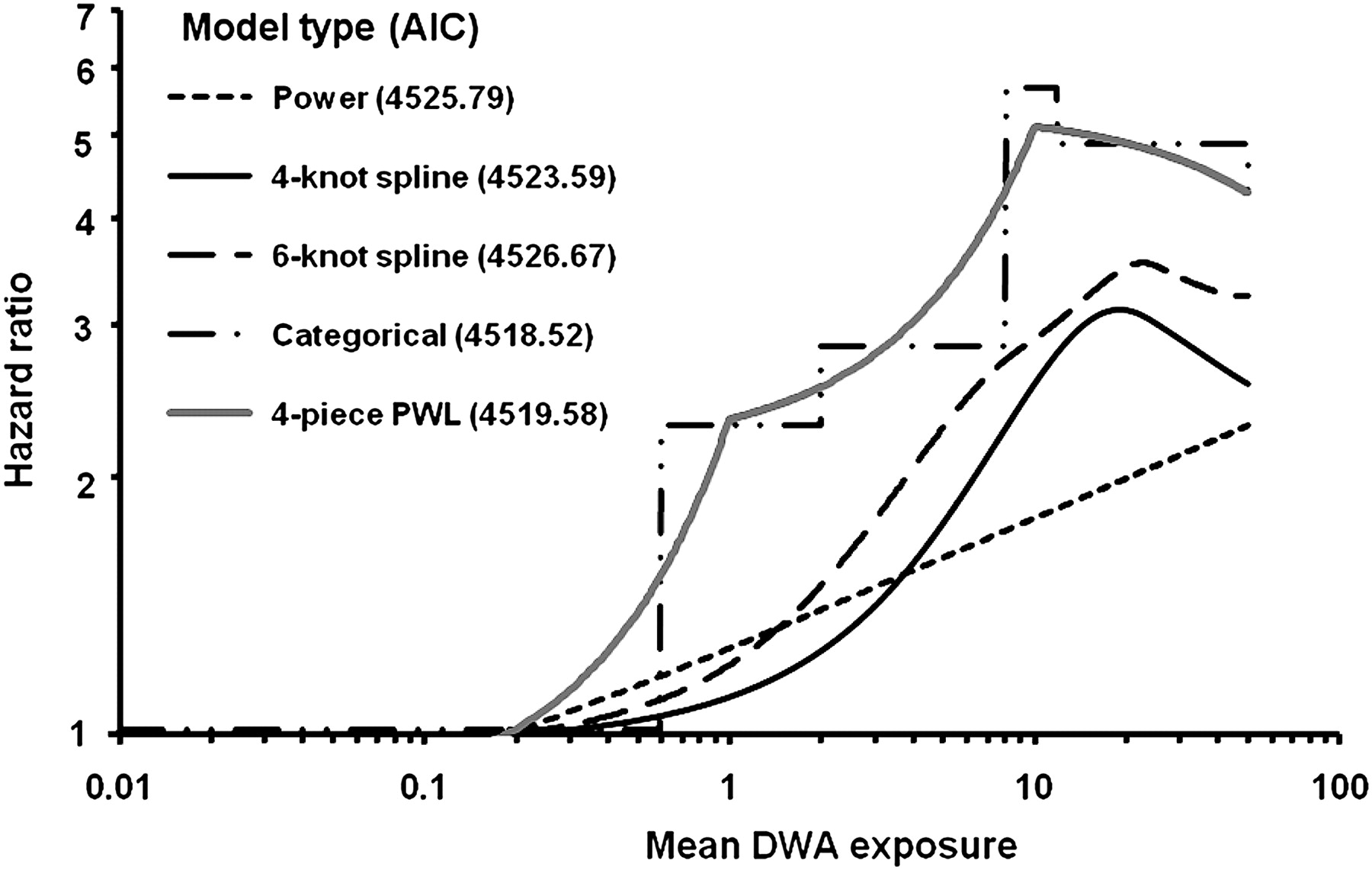
The categorical model (with reference category 0–<0.6 μg/m3) and the four-piece piecewise log-linear model provided the best exposure–response fit for mean exposure. Figure 1 shows the power model and the four- and six-knot restricted cubic splines, compared with the best-fitting models, for mean exposure. Except for the power model, all fits have similar shapes.

Comparison of fit of different dose–response models (spline, best-fitting categorical, power, four-piece log-linear) for mean ‘daily weighted average’ (DWA) exposure, adjusting for birth cohort and plant and normalised to the mean (0.185 μg/m3) of the baseline group in the categorical model. AIC, Akaike Information Criterion value; PWL, piecewise log-linear.
The coefficients for the best-fitting piecewise log-linear models for mean, maximum and cumulative exposure are given in table 3. Beta coefficients are also shown in table 3 excluding asbestos-exposed and professional workers. The steepest increase in lung cancer risk was between 0 and 0.8 μg/m3 for mean exposure, between 0 and 1 μg/m3 for maximum exposure and between 0 and 200 μg/m3-days for cumulative exposure. For mean exposure, a model with cutpoints at 1.0 fitted nearly as well, demonstrated a monotonic increase in risk between 0 and 2 μg/m3, and included at least 20 cases below the lowest cutpoint. Thus, it was deemed more suitable for risk calculations, and coefficients for this model are given in online appendix table 6.
Best piecewise log-linear coefficients for 10-year-lagged mean, maximum and cumulative ‘daily weighted average’ (DWA) exposure final models
Likelihood ratio χ2 tests of this mean DWA PWL model indicated that the set of β coefficients was highly significant for a model using all workers (deviance χ2=29.83, df=4, p=5.3e–6) and for a model excluding asbestos-exposed and professionals (deviance χ2=27.92, df=4, p=1.3e–5).
The PWL model for mean exposure produced HRs significantly greater than one at all exposure levels when all workers were included in the model, and at exposures at about 4 μg/m3 and above when professionals and asbestos-exposed workers were excluded (See online appendix table 7). HRs were slightly higher at the same exposure level for maximum compared with mean DWA across most of the range of exposure values, although when excluding asbestos and professional workers, significantly elevated HRs were observed only above 10 μg/m3. For cumulative exposure, HRs were significantly greater than 1 at all exposure levels under both conditions.
Risk assessment calculations
The lifetime male background risk of lung cancer mortality (assuming survival to age 30) was estimated to be 0.0664. In models including all workers, the estimated HR at a mean DWA beryllium exposure of 0.5 μg/m3 (the NIOSH recommended exposure limit) ranged from 1.11 in the categorical model (estimated using the category 2.0–8 μg/m3) to 1.68 in the PWL model (table 4). When excluding professionals and workers with potential asbestos exposure, the estimated HR at 0.5 μg/m3 ranged from 1.09 for the categorical model to 1.74 for the power model. These were associated with estimates of lifetime excess absolute risk ranging from 0.0061 to 0.049 (table 4).
Estimated hazard ratio (HR) and excess absolute risk (EAR) for a mean ‘daily weighted average’ (DWA) exposure at the National Institute for Occupational Safety and Health recommended exposure limit of 0.5 μg/m3, and mean DWA exposure associated with 10−3 EAR, under different assumed exposure–response models
The mean DWA beryllium exposure associated with 10−3 lifetime excess lung cancer mortality risk based on US male population rates (for a model including all workers) ranged from 0.0050 μg/m3 for HRs from the power model to 0.070 μg/m3 for those from the categorical model (table 4). When excluding professionals and those potentially exposed to asbestos, the corresponding exposure levels were slightly lower for the power model and slightly higher for the categorical and PWL models. The best-fitting PWL among these workers produced a 10−3 lifetime excess risk estimate at 0.033 μg/m3 (table 4).
Discussion
We found that lung cancer risk was significantly and strongly related to mean, maximum and cumulative exposure, when considering a variety of potential confounders related to likely smoking behaviour and potential exposure to other lung carcinogens. These findings extend those of the nested case–control study previously conducted for the Reading facility.6 7 Compared with the most recent results reported for this facility, we observed generally higher beryllium-associated risks in the categorical and power models. Some increase in precision was due to the additional 13 years of follow-up. The inclusion of data for the two smaller plants (Elmore and Hazleton) also contributed important information about risk at low exposure, as the majority of these subjects had mean DWA exposures lower than 2 μg/m3.
Other differences among the facilities provide context for the findings observed here; the Reading plant began operations in the 1930s, while Elmore and Hazleton began in the 1950s.4 Reading plant workers were born earlier, on average (1917), than Elmore and Hazleton plant workers (1931 and 1935, respectively5). In the previous Reading plant study,7 a significant interaction was observed between mean DWA exposure and birth cohort: workers born before 1900 had a higher beryllium-associated lung cancer risk than workers born later and also tended to have lower lagged exposure than workers born later. In the present study, we observed no interaction between 10-year-lagged mean DWA exposure and birth cohort in producing lung cancer. This change is likely due to the inclusion of the Elmore and Hazleton plants, which provide exposure–response information at low exposures for later birth cohorts.
Adjustment for plant as a confounder was important for this pooled study: this is likely due to the large differences by plant in exposure levels and demographic characteristics, as well as the lower age-adjusted background lung cancer rate in Berks County (PA), the location of the Reading plant, compared with those in Ottawa (OH) and Luzerne (PA) counties, where the other two plants are located.22
The estimated HRs per unit exposure for mean and maximum DWA exposure were very similar, as were the power model β coefficients. This finding is consistent with the method by which these metrics were calculated: mean DWA exposure represents a mean exposure over a working lifetime (up to the cut-off date) of the annual average job exposures. These annual average job exposures were the geometric means of up to four quarterly estimates. The maximum exposure was the highest annual average job exposure a worker experienced through the cut-off date. Our findings of similar (but slightly higher) risk per unit exposure for maximum compared with mean exposure may reflect the similarity of these two metrics for individual workers.
Spline models have been recommended for identifying good-fitting parametric models that may be useful for risk-assessment purposes.18 23 Our empirically fitted restricted cubic spline models described lung cancer HRs that increased steeply at mean and maximum exposures below about 10 μg/m3 and then attenuated above that. This corresponds well to the results produced by the best-fitting categorical model, and the pattern is also well fitted by the PWL and power models. PWL models may be more suitable for risk projections at low exposures than the power models employed here and in previous analyses,6 7 as the latter produce very high risk estimates at low exposures, where the data are sparse. The attenuation we observed in HRs at higher exposure is commonly observed in occupational studies24 and may be caused by exposure misclassification that is proportional to exposure, the healthy worker survivor effect, depletion of susceptible individuals from the source population or differences in exposure rate effects by cumulative exposure level.
Strengths of this study include the lengthy follow-up of the cohort hired between plant construction and 1970, the pooling and use of a common protocol to analyse data for all three plants, and, especially, the availability of exposure and employment data with which to develop quantitative estimates of exposure for each worker. The beryllium exposure monitoring information for all three plants was extensive, consisting of thousands of measurements collected consistently both across each plant and over decades of use of the metal. In addition, information from plant monitoring sources has been independently evaluated against concurrent measurements collected by the Atomic Energy Commission.25 Another study strength is its consideration of potentially confounding exposures to other lung carcinogens, including acid mist, asbestos, cadmium, chromium, nickel and silica. These determinations were made on a job-specific basis, and the information was integrated over the entire plant employment history of each worker. We found that these exposures, with the possible exception of asbestos, had little impact on the risk estimates associated with beryllium exposure. Excluding workers with the potential for asbestos exposure also did not greatly affect estimated lung cancer risk associated with low beryllium exposure.
This study also has a number of limitations. Smoking information was available only for a subset of the cohort (ie, those employed in 1968). New analyses of these smoking data indicate that the workers smoked at comparable levels to the overall US population.5 There were slightly fewer heavy smokers and more never- and former-smokers in the cohort than in the US population. The same analyses indicate that there is little difference within the cohort in smoking by cumulative or maximum exposure category. In the current analysis, adjustment for a likely smoking surrogate—professional employment status—had little impact on risk estimates, low-exposure curve-fitting (tables 2 and 3) or the predicted risks at low exposure levels (table 4). Furthermore, other studies have found that internal analyses are less likely to be confounded by smoking differences,26 and within-cohort risk ratios of greater than 1.5 are unlikely to be explained by smoking differences.27 28
There are also some limitations related to the available exposure metrics. As described above, we did not have information on weekly or monthly variation in exposure. Although the use of time-integrated metrics in conjunction with studies of chronic beryllium disease has been criticised,29 the mean working lifetime DWA exposure level, in particular, may provide a useful representation of the exposure intensity over an entire working lifetime, and we note that the American Conference of Governmental Industrial Hygienists recommends the use of such long-term averages in its new threshold limit value-time weighted average for beryllium.30 This metric also should prove useful for evaluation of lifetime risk associated with beryllium exposure, as we have calculated here.
The JEMs we employed did not assume that use of respirators resulted in respiratory protection.13–15 This may have led to an overestimate of exposure, which may have been more severe for the more highly exposed workers. This could explain the attenuation in risk at high exposures, as upward exposure misclassification was likely greater at higher exposure levels.
Recently, the long-practised use of age-based risk set sampling in conjunction with exposure lagging has been criticised.31 32 Levy and colleagues32 proposed that controls sampled from age-based risk sets should be matched on the age at date of last observation in order to correct a supposed ‘imbalance’ between cases and controls. Theoretical considerations33 34 question this new matching criterion, and empirical simulations12 35 implementing it have found that it produces a notable downward bias in risk estimates. Wacholder36 notes that traditional risk set sampling is expected to produce unbiased results, even when exposure lagging is used. Another simulation study, which takes into account birth cohort effects observed in the Reading cohort, confirmed this37 and also found that finer adjustment for birth year affected results little. The present study, although not a case–control study, used age-based full risk sets calculated in the typical method. In contrast to our previous analyses of the Reading nested case–control study,7 we observed that shorter lags produced very similar estimates to those of the 10-year lags, although the latter fitted the data better.
Conclusion
We found that lung cancer risk is statistically significantly elevated at 4 μg/m3 DWA, very near the current US Occupational Safety and Health Administration exposure limit of 2 μg/m3 DWA for workers. Risk projections at lower exposures indicate that mean DWA exposure associated with a one-in-one-thousand excess lifetime risk of lung cancer mortality is approximately 0.033 μg/m3. This level is 60 times lower than the current Occupational Safety and Health Administration permissible exposure limit,38 15 times lower than the current NIOSH recommended exposure limit,9 and just under the 0.05 μg/m3 ‘threshold limit value-time-weighted average’ (based on prevention of beryllium sensitisation and chronic beryllium disease) recently adopted by the American Conference of Governmental Industrial Hygienists.30 The parameter estimates from these analyses should prove useful for groups interested in producing quantitative risk estimates of lung cancer following beryllium exposure.39
Acknowledgments
The authors thank S Allee, S Bertke and K Waters, for providing computer-programming support for this project; M Hein, for discussions on the effects of different birth year adjustment methods; and D Kriebel, J Lubin and D Richardson, for helpful comments on the manuscript.
References
Footnotes
Funding Funding for this study was provided by the US National Institute for Occupational Safety and Health.
Competing interests None.
Ethics approval Ethics approval was provided by the National Institute for Occupational Safety and Health Human Subjects Review Board.
Provenance and peer review Not commissioned; externally peer reviewed.